Joins for tables

dplyr

Aurélien Ginolhac

University of Luxembourg

Friday, the 25^th of April, 2025

Relational operations

Combining data from two tables

How do we refer to a particular observation?

Primary key

The column that uniquely identifies an observation

• Frequently an ID
• Can be introduced by row_number() if no primary column exists bona fide observations

Composite key

Several columns that together identify an observation uniquely to serve as primary key.

Like patient and visit

Foreign key

A key referring to observations in another table

Your turn!

Which columns are keys?

• In judgments

judge_url <- "https://biostat2.uni.lu/practicals/data/judgments.tsv"
judgments <- read_tsv(judge_url, show_col_types = FALSE)

• In datasauRus::datasaurus_dozen
• In swiss

Warning

Tibbles do not have row names! Frequently these are the primary keys!

Use as_tibble(data, rownames = "ID") for swiss

03:00

Solution

swiss: Province is primary key.

Once you took care of the rownames.

as_tibble(swiss, 
          rownames = "Province")

# A tibble: 47 × 7
   Province     Fertility Agriculture Examination Education Catholic
   <chr>            <dbl>       <dbl>       <int>     <int>    <dbl>
 1 Courtelary        80.2        17            15        12     9.96
 2 Delemont          83.1        45.1           6         9    84.8 
 3 Franches-Mnt      92.5        39.7           5         5    93.4 
 4 Moutier           85.8        36.5          12         7    33.8 
 5 Neuveville        76.9        43.5          17        15     5.16
 6 Porrentruy        76.1        35.3           9         7    90.6 
 7 Broye             83.8        70.2          16         7    92.8 
 8 Glane             92.4        67.8          14         8    97.2 
 9 Gruyere           82.4        53.3          12         7    97.7 
10 Sarine            82.9        45.2          16        13    91.4 
# ℹ 37 more rows
# ℹ 1 more variable: Infant.Mortality <dbl>

Datasaurus: composite key from all the variables

sample_n(datasauRus::datasaurus_dozen, 5)

# A tibble: 5 × 3
  dataset        x     y
  <chr>      <dbl> <dbl>
1 wide_lines  67.5 16.4 
2 v_lines     30.5 49.4 
3 high_lines  58.5 81.7 
4 bullseye    53.0  9.91
5 v_lines     50.2 73.1 

Or a primary key from row numbers

as_tibble(datasauRus::datasaurus_dozen, 
          rownames = "ID")

# A tibble: 1,846 × 4
   ID    dataset     x     y
   <chr> <chr>   <dbl> <dbl>
 1 1     dino     55.4  97.2
 2 2     dino     51.5  96.0
 3 3     dino     46.2  94.5
 4 4     dino     42.8  91.4
 5 5     dino     40.8  88.3
 6 6     dino     38.7  84.9
 7 7     dino     35.6  79.9
 8 8     dino     33.1  77.6
 9 9     dino     29.0  74.5
10 10    dino     26.2  71.4
# ℹ 1,836 more rows

Primary key in judgments

Should be subject

select(judgments, subject)

# A tibble: 188 × 1
   subject
     <dbl>
 1       2
 2       1
 3       3
 4       4
 5       7
 6       6
 7       5
 8       9
 9      16
10      13
# ℹ 178 more rows

But really?

count(judgments, subject, sort = TRUE) |> 
  slice_head(n = 3)

# A tibble: 3 × 2
  subject     n
    <dbl> <int>
1      75     2
2       1     1
3       2     1

What is going on for subject 75?

Matching subjects between two tibbles

Additional data for some participants

• Coffee consumption

tribble(~student, ~coffee_shots, 
        21,       1,
        23,       4,
1        211,      3,
        28,       2) -> coffee_drinkers
coffee_drinkers

1

Not present in the initial data

# A tibble: 4 × 2
  student coffee_shots
    <dbl>        <dbl>
1      21            1
2      23            4
3     211            3
4      28            2

Smaller sample set

subject_mood <- judgments |>
  select(subject, condition, gender, 
         starts_with("mood")) |> 
  distinct() # for issue with subject 75
subject_mood

# A tibble: 187 × 5
   subject condition gender mood_pre mood_post
     <dbl> <chr>     <chr>     <dbl>     <dbl>
 1       2 control   female       81        NA
 2       1 stress    female       59        42
 3       3 stress    female       22        60
 4       4 stress    female       53        68
 5       7 control   female       48        NA
 6       6 stress    female       73        73
 7       5 control   female       NA        NA
 8       9 control   male        100        NA
 9      16 stress    female       67        74
10      13 stress    female       30        68
# ℹ 177 more rows

Goal: Add coffee consumption

Combining the two tables

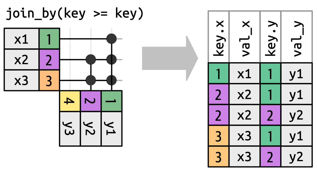
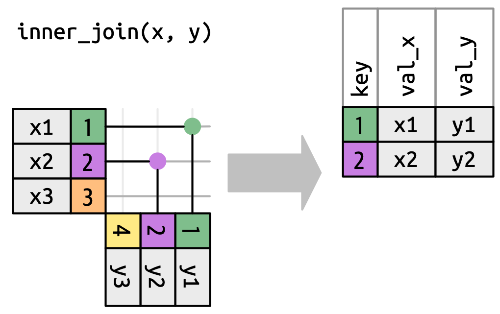
Inner join

Error! no common key.

inner_join(coffee_drinkers, 
           subject_mood)

Error in `inner_join()`:
! `by` must be supplied when `x` and `y` have no common variables.
ℹ Use `cross_join()` to perform a cross-join.

Provide the correspondences

inner_join(coffee_drinkers,
           subject_mood,
           by = join_by(student == subject))

# A tibble: 3 × 6
  student coffee_shots condition gender mood_pre mood_post
    <dbl>        <dbl> <chr>     <chr>     <dbl>     <dbl>
1      21            1 control   female       68        NA
2      23            4 control   female       78        NA
3      28            2 stress    male         53        68

Initial tables are not preserved, but mutated

Mutating joins

Creating new tables through joins

• Key operations in data processing
• inner_join() is the most strict join operations
• left_join() focuses on left table
• right_join() focuses on right table
• full_join() joins both tables
• Missing values can create massive matches
• left, right, full create missing values for unmatched rows

Join types

From the by = argument and specified in the join_by() helper:

• Equality joins (==)
• Inequality joins (>=)
• Rolling joins (closest(a >= b))
• Overlap joins (between() / within() / overlaps())
• Cross joins, returns Cartesian product nrow(x) * nrow(y)

Mutating joins, overview

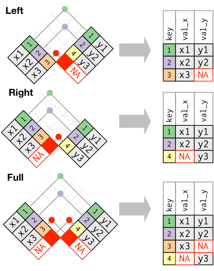
Left join

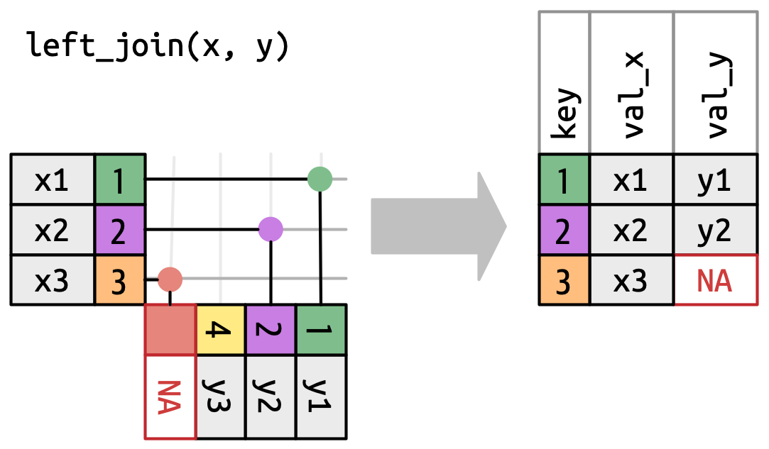
Left tibble keeps same numbers of rows.

Example with left_join()

left_join(subject_mood, coffee_drinkers, 
          by = join_by(subject == student))

# A tibble: 187 × 6
   subject condition gender mood_pre mood_post coffee_shots
     <dbl> <chr>     <chr>     <dbl>     <dbl>        <dbl>
 1       2 control   female       81        NA           NA
 2       1 stress    female       59        42           NA
 3       3 stress    female       22        60           NA
 4       4 stress    female       53        68           NA
 5       7 control   female       48        NA           NA
 6       6 stress    female       73        73           NA
 7       5 control   female       NA        NA           NA
 8       9 control   male        100        NA           NA
 9      16 stress    female       67        74           NA
10      13 stress    female       30        68           NA
# ℹ 177 more rows

The missing subject 211 is unmatched and not returned

left_join(subject_mood, coffee_drinkers, 
          by = join_by(subject == student)) |> 
  filter(!is.na(coffee_shots))

# A tibble: 3 × 6
  subject condition gender mood_pre mood_post coffee_shots
    <dbl> <chr>     <chr>     <dbl>     <dbl>        <dbl>
1      23 control   female       78        NA            4
2      21 control   female       68        NA            1
3      28 stress    male         53        68            2

Right-join

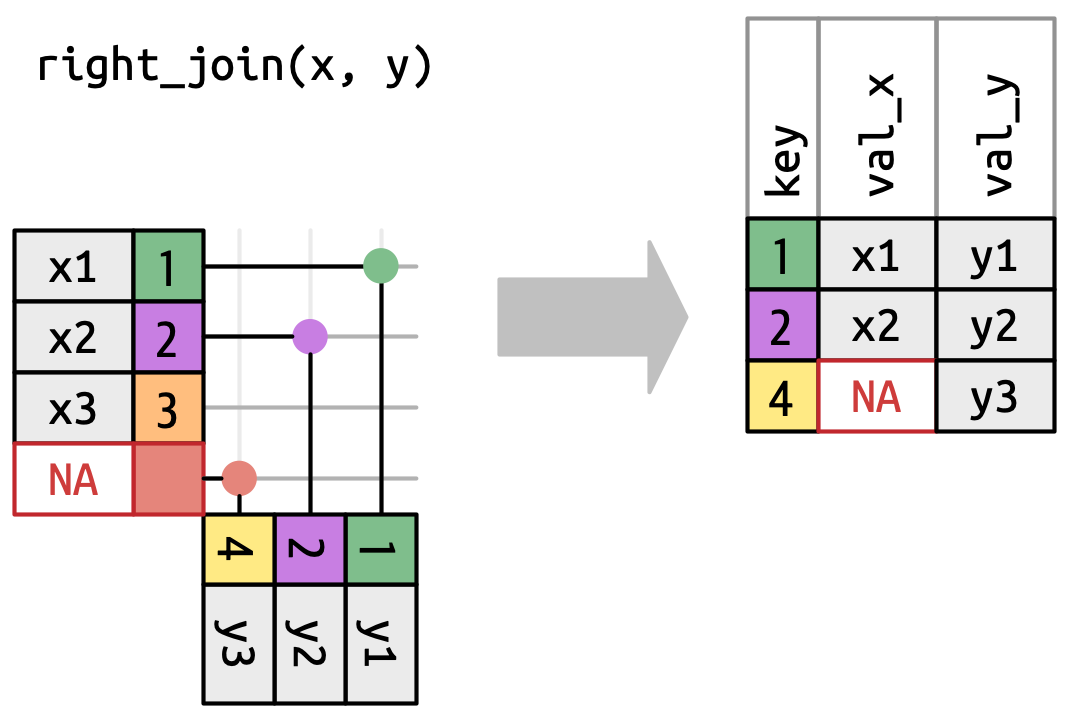
Right tibble matters

Example with right_join()

right_join(subject_mood, coffee_drinkers, 
           by = join_by(subject == student))

# A tibble: 4 × 6
  subject condition gender mood_pre mood_post coffee_shots
    <dbl> <chr>     <chr>     <dbl>     <dbl>        <dbl>
1      23 control   female       78        NA            4
2      21 control   female       68        NA            1
3      28 stress    male         53        68            2
4     211 <NA>      <NA>         NA        NA            3

The missing subject 211 is unmatched and returned with NA for left columns

Full-join

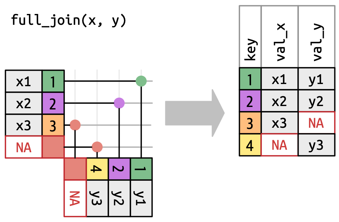
Number of rows = left + right

Example with full_join()

full_join(subject_mood, coffee_drinkers, 
          by = join_by(subject == student))

# A tibble: 188 × 6
   subject condition gender mood_pre mood_post coffee_shots
     <dbl> <chr>     <chr>     <dbl>     <dbl>        <dbl>
 1       2 control   female       81        NA           NA
 2       1 stress    female       59        42           NA
 3       3 stress    female       22        60           NA
 4       4 stress    female       53        68           NA
 5       7 control   female       48        NA           NA
 6       6 stress    female       73        73           NA
 7       5 control   female       NA        NA           NA
 8       9 control   male        100        NA           NA
 9      16 stress    female       67        74           NA
10      13 stress    female       30        68           NA
# ℹ 178 more rows

The missing subject 211 is unmatched and returned with NAs

full_join(subject_mood, coffee_drinkers, 
          by = join_by(subject == student)) |> 
  filter(!is.na(coffee_shots))

# A tibble: 4 × 6
  subject condition gender mood_pre mood_post coffee_shots
    <dbl> <chr>     <chr>     <dbl>     <dbl>        <dbl>
1      23 control   female       78        NA            4
2      21 control   female       68        NA            1
3      28 stress    male         53        68            2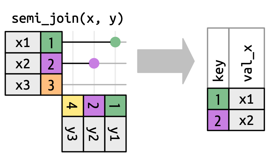
4     211 <NA>      <NA>         NA        NA            3

Two tables - same column names

What if we have gender in both tables?

coffee_drinkers <- mutate(coffee_drinkers, 
                          gender = c("female", "female", 
                                     "male", "male"))
coffee_drinkers

# A tibble: 4 × 3
  student coffee_shots gender
    <dbl>        <dbl> <chr> 
1      21            1 female
2      23            4 female
3     211            3 male  
4      28            2 male  

1. Add this column gender to the joins

left_join(subject_mood,
          coffee_drinkers,
          by = join_by(gender, subject == student))

# A tibble: 187 × 6
   subject condition gender mood_pre mood_post coffee_shots
     <dbl> <chr>     <chr>     <dbl>     <dbl>        <dbl>
 1       2 control   female       81        NA           NA
 2       1 stress    female       59        42           NA
 3       3 stress    female       22        60           NA
 4       4 stress    female       53        68           NA
 5       7 control   female       48        NA           NA
 6       6 stress    female       73        73           NA
 7       5 control   female       NA        NA           NA
 8       9 control   male        100        NA           NA
 9      16 stress    female       67        74           NA
10      13 stress    female       30        68           NA
# ℹ 177 more rows

2. Exclude gender, col names are kept and added suffixes - .x and .y

left_join(subject_mood,
          coffee_drinkers,
          by = join_by(subject == student)) |> 
  relocate(starts_with("gender"), coffee_shots) |> 
  arrange(desc(coffee_shots))

# A tibble: 187 × 7
   gender.x gender.y coffee_shots subject condition mood_pre mood_post
   <chr>    <chr>           <dbl>   <dbl> <chr>        <dbl>     <dbl>
 1 female   female              4      23 control         78        NA
 2 male     male                2      28 stress          53        68
 3 female   female              1      21 control         68        NA
 4 female   <NA>               NA       2 control         81        NA
 5 female   <NA>               NA       1 stress          59        42
 6 female   <NA>               NA       3 stress          22        60
 7 female   <NA>               NA       4 stress          53        68
 8 female   <NA>               NA       7 control         48        NA
 9 female   <NA>               NA       6 stress          73        73
10 female   <NA>               NA       5 control         NA        NA
# ℹ 177 more rows

Two tables - same column names

Remark

Suffixes for columns with the same name can be controlled.

Join by one column

left_join(subject_mood,
          coffee_drinkers,
          by = join_by(subject == student),
          suffix = c( "_mood", "_coffee")) |>
  relocate(starts_with("gender"), coffee_shots) |> 
  arrange(desc(coffee_shots))

# A tibble: 187 × 7
   gender_mood gender_coffee coffee_shots subject condition mood_pre mood_post
   <chr>       <chr>                <dbl>   <dbl> <chr>        <dbl>     <dbl>
 1 female      female                   4      23 control         78        NA
 2 male        male                     2      28 stress          53        68
 3 female      female                   1      21 control         68        NA
 4 female      <NA>                    NA       2 control         81        NA
 5 female      <NA>                    NA       1 stress          59        42
 6 female      <NA>                    NA       3 stress          22        60
 7 female      <NA>                    NA       4 stress          53        68
 8 female      <NA>                    NA       7 control         48        NA
 9 female      <NA>                    NA       6 stress          73        73
10 female      <NA>                    NA       5 control         NA        NA
# ℹ 177 more rows

Filtering joins

Only the existence of a match is important; it doesn’t matter which observation is matched. This means that filtering joins never duplicate rows like mutating joins do

— Hadley Wickam

Filter matches in x, no duplicates

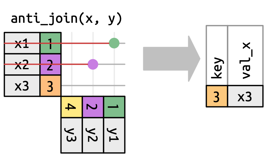
Extract what does not match

semi_join() does not alter original

(tx <- tribble(~key, ~x,
              1, "x1", 
              2, "x2", 
              3, "x3", 
              4, "x4"))

# A tibble: 4 × 2
    key x    
  <dbl> <chr>
1     1 x1   
2     2 x2   
3     3 x3   
4     4 x4   

(ty <- tribble(~key, ~y,
              1, "y1",
              2, "y2",
              2, "y3",
              3, "y4"))

# A tibble: 4 × 2
    key y    
  <dbl> <chr>
1     1 y1   
2     2 y2   
3     2 y3   
4     3 y4   

Filtering

semi_join(tx, ty)

Joining with `by = join_by(key)`

# A tibble: 3 × 2
    key x    
  <dbl> <chr>
1     1 x1   
2     2 x2   
3     3 x3   

Mutating

inner_join(tx, ty)

Joining with `by = join_by(key)`

# A tibble: 4 × 3
    key x     y    
  <dbl> <chr> <chr>
1     1 x1    y1   
2     2 x2    y2   
3     2 x2    y3   
4     3 x3    y4   

When by = not precised, cols are reported (here, means key == key)

Cross join, Cartesian product

For permutations

tib <- tibble(name = c("John", "Simon", 
                       "Tracy", "Max"))
cross_join(tib, tib)

# A tibble: 16 × 2
   name.x name.y
   <chr>  <chr> 
 1 John   John  
 2 John   Simon 
 3 John   Tracy 
 4 John   Max   
 5 Simon  John  
 6 Simon  Simon 
 7 Simon  Tracy 
 8 Simon  Max   
 9 Tracy  John  
10 Tracy  Simon 
11 Tracy  Tracy 
12 Tracy  Max   
13 Max    John  
14 Max    Simon 
15 Max    Tracy 
16 Max    Max   

Non-equi joins

tib <- tibble(id = 1:4, name = c("John", "Simon", 
                                 "Tracy", "Max"))
left_join(tib, tib, join_by(id < id))

# A tibble: 7 × 4
   id.x name.x  id.y name.y
  <int> <chr>  <int> <chr> 
1     1 John       2 Simon 
2     1 John       3 Tracy 
3     1 John       4 Max   
4     2 Simon      3 Tracy 
5     2 Simon      4 Max   
6     3 Tracy      4 Max   
7     4 Max       NA <NA>  

Rolling joins

tib <- tibble(id = 1:4, name = c("John", "Simon", 
                                 "Tracy", "Max"))
left_join(tib, tib, join_by(closest(id < id)))

# A tibble: 4 × 4
   id.x name.x  id.y name.y
  <int> <chr>  <int> <chr> 
1     1 John       2 Simon 
2     2 Simon      3 Tracy 
3     3 Tracy      4 Max   
4     4 Max       NA <NA>  

Helpful tools

Removing the data frame context through pull()

Remark

By default tidyverse operations that receive a tibble as input return a tibble.

Extract column by name as vector

pull(judgments, age)[1:10]

 [1] 24 19 19 22 22 22 18 20 21 19

Extract same vector along with names

pull(judgments, age, name = subject)[1:10]

 2  1  3  4  7  6  5  9 16 13 
24 19 19 22 22 22 18 20 21 19 

Comparing to data in other rows

Leading and lagging rows

• lead() for data in following row
• lag() for data in the row above

Calculate differences between subjects

Let’s assume the subject IDs are in order of the tests being conducted. What is the difference to the previous subject for the “initial mood”?

judgments |>
  select(subject, mood_pre) |> 
  arrange(subject) |> 
  mutate(prev_mood_pre = lag(mood_pre),
         mood_diff = mood_pre - lag(mood_pre))

# A tibble: 188 × 4
   subject mood_pre prev_mood_pre mood_diff
     <dbl>    <dbl>         <dbl>     <dbl>
 1       1       59            NA        NA
 2       2       81            59        22
 3       3       22            81       -59
 4       4       53            22        31
 5       5       NA            53        NA
 6       6       73            NA        NA
 7       7       48            73       -25
 8       8       59            48        11
 9       9      100            59        41
10      10       72           100       -28
# ℹ 178 more rows

The other 20% of dplyr

Occasionally handy

• Assembly: bind_rows, bind_cols
• Windows function, min_rank, dense_rank, cumsum. See - vignette
• Working with list-columns (courses next year)
• multidplyr for parallelized code

SQL mapping allows database access

• dplyr code can be translated into SQL and query databases online (using dbplyr)
• Different types of tabular data (dplyr SQL backend, databases,

Before we stop

You learned to:

• Joining and intersecting tibbles
• Differ filtering from mutation joins

Acknowledgments 🙏 👏

• Hadley Wickham
• Lionel Henry
• Romain François
• Allison Horst for the great ArtWork
• Jenny Bryan

Contributions

• Milena Zizovic
• Roland Krause

Thank you for your attention!