```{r}
#| label: readin-csv
#| code-line-numbers: false
#| eval: false
# regular comment, not a hash pipe
wine <- read_csv("wine.tsv")
```Quarto
Literate programming
Monday 9 Mar, 2026
Learning objectives
You will learn to:

- How to structure files and folders
- Use relative paths and RStudio projects
- Use the markdown syntax
- Create Quarto documents
- Render to the output format you want
- Use RStudio interface to
- Create your documents
- Insert R code
- Build your final document
Organize your files
Absolute paths are NOT portable
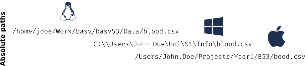
Relative paths are
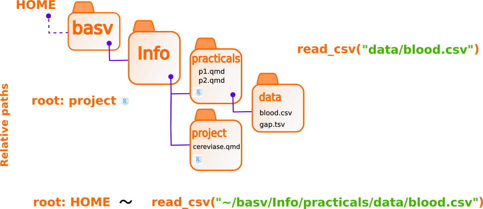
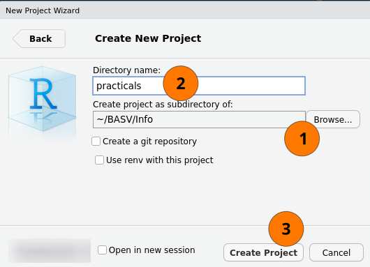
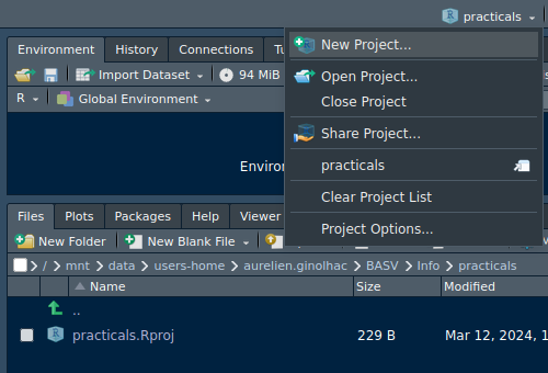
RStudio projects
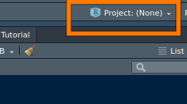
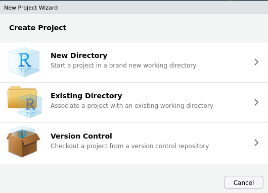
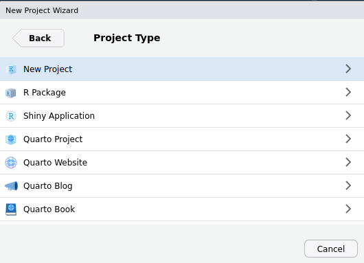
Create the practicals RStudio project
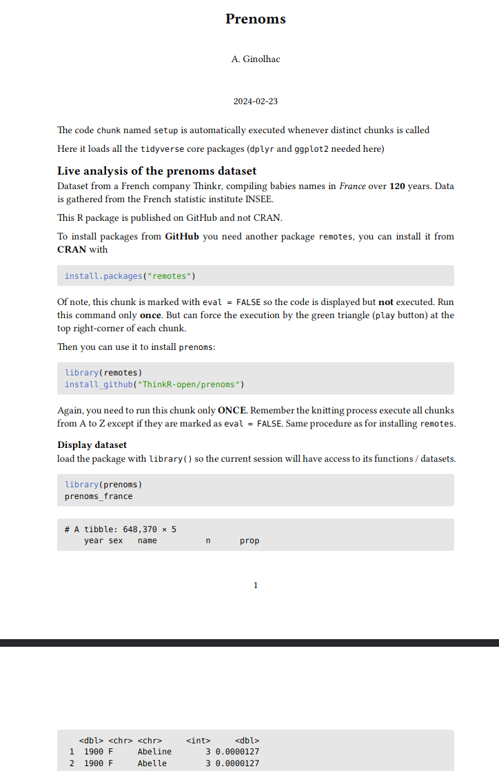
Rmarkdown
Predecessor of Quarto. Files are .Rmd.
Version 1 in 2016, the idea was to have text and code in one document, execute code and let the final markdown converted to different formats by pandoc.
Quarto
Extended Rmarkdown. Languages and IDE agnostic

Markdown, lightweight markup language with a simple syntax
- Started 2004 by John Gruber
- Hyper Text Markup Language=HTML How Markdown took over the world by Anil Dash
If mark up is complicated, then the opposite of that complexity must be… mark down.
HTML
<!DOCTYPE html>
<html>
<body>

<h1>This is a heading</h1>

<p>This is some text in a <b>paragraph</b></p>

<h2>This is a second level heading</h2>

<ul>
<li><a href="http://exa.com"><code>site</code></a>
<li><img src="https://images.computerhistory.org/revonline/images/500004391-03-01.jpg?w=200">
</ul>
</body>
</html>
Markdown equivalent
# This is a heading
This is some text in a **paragraph**
## This is a second level heading
- [`site`](http://exa.com)
- 
Including code to execute
Quarto document: Structure

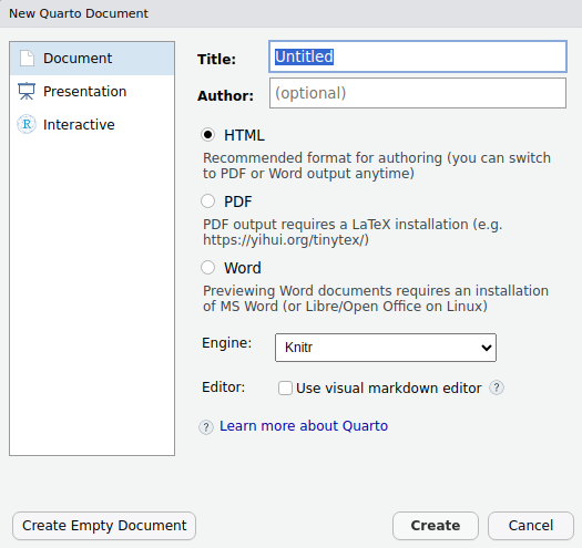
Qmd creation: step 1
Under File, pick Quarto Document
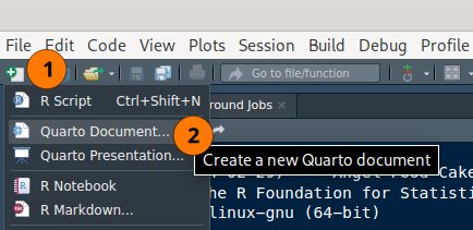
- Optionally fill in some header variables
- Choose the output format (can be changed later)
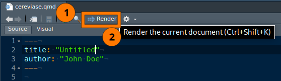
Render Quarto documents
- Save the file,
Untitled.qmd*cannot be rendered - Click the Render
- A new session is created
- Chunks are evaluated top -> bottom
- Outputs are injected in the MD
- Final MD is converted by
pandocto chosenformat: pdf
Example:
---
title: "Cereviase"
format: pdf
---
Default output is HTML
code chunks
Insert a chunk
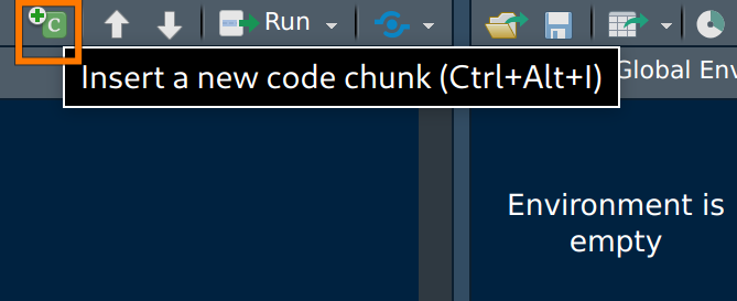
Basic Markup
- Delimited by triple backticks tags (
```) - Engine evaluating the code in curly braces
- Options in hash pipe:
#|- Label of chunk (optional)
- Show/hide code
#| echo: true - Evaluate or not
#| eval: true - Figure size (inches)
#| fig-width: 9 - …
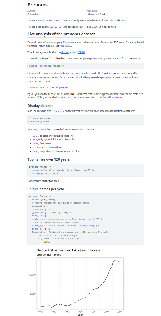
Output examples 1/2
HTML
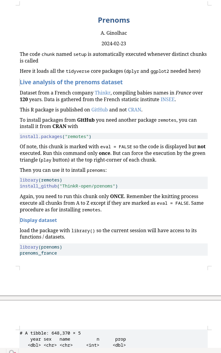
Word
Output examples 2/2
Typst
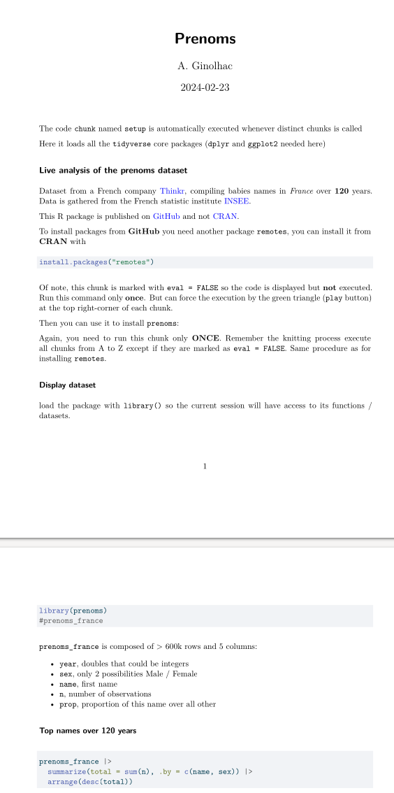
PDF (LaTex)