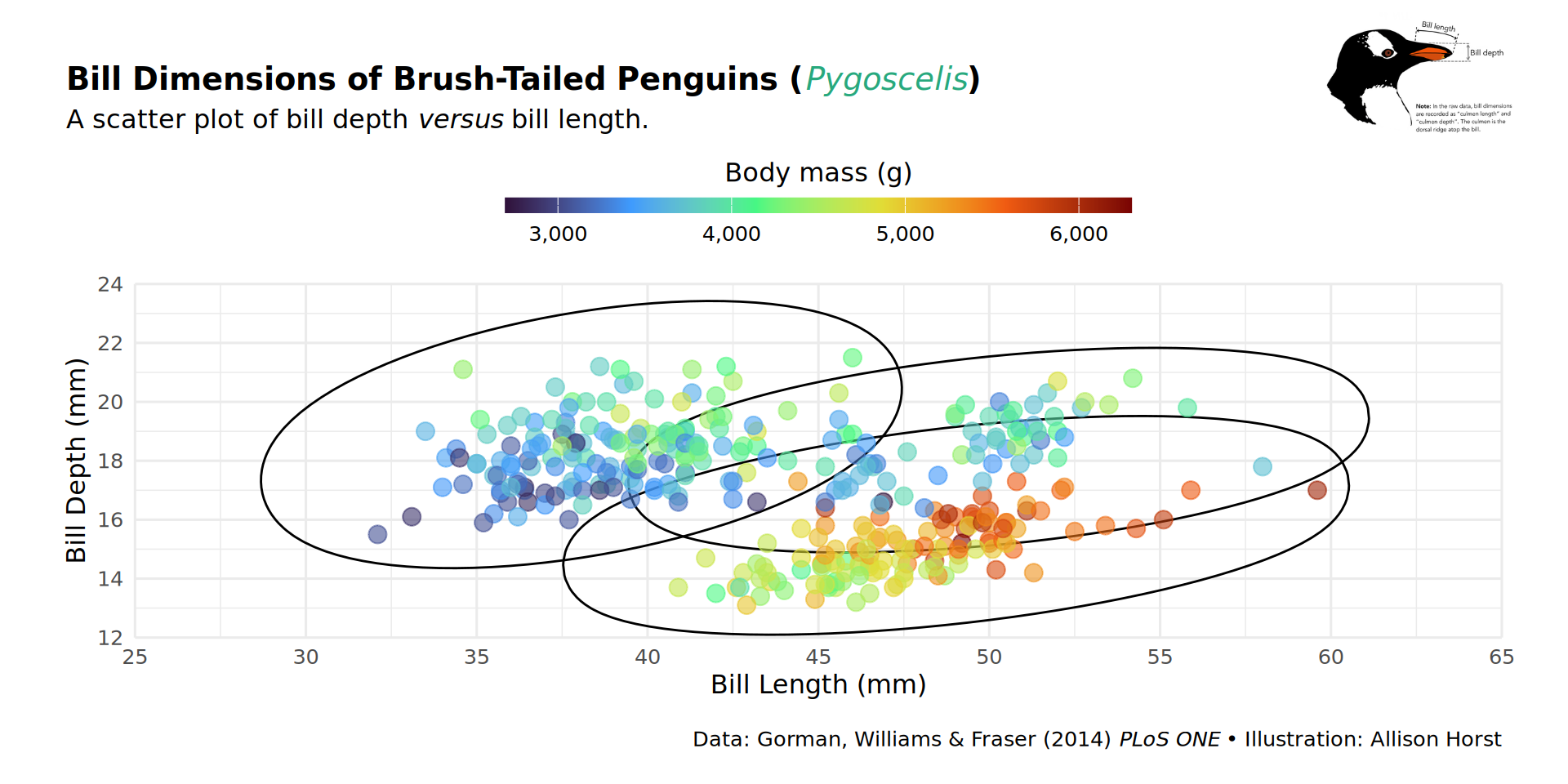
culmen <- png::readPNG("img/plot_culmen_depth.png", native = TRUE)
penguins |>
filter_out(if_any(starts_with("bill"), is.na)) |>
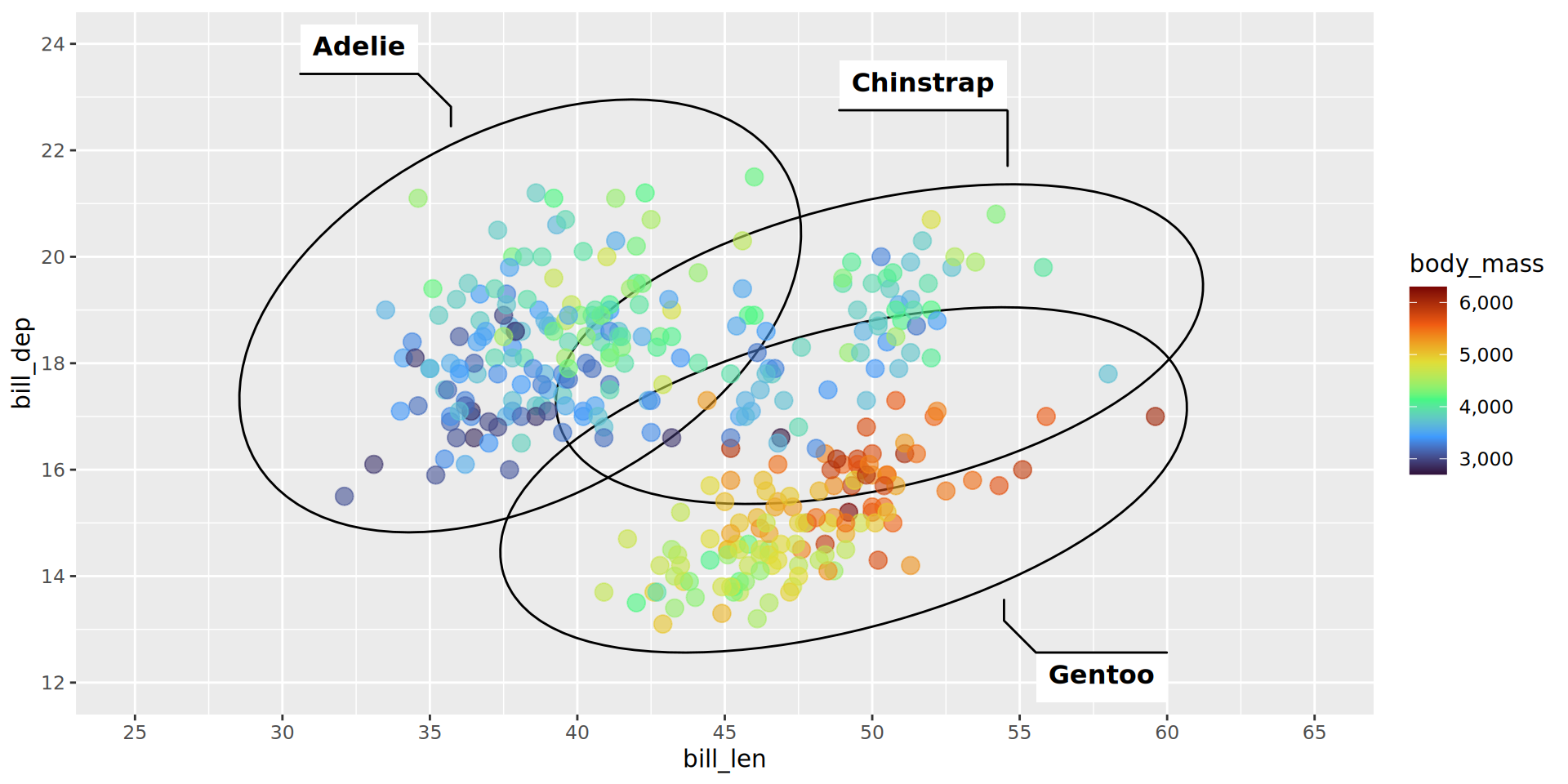
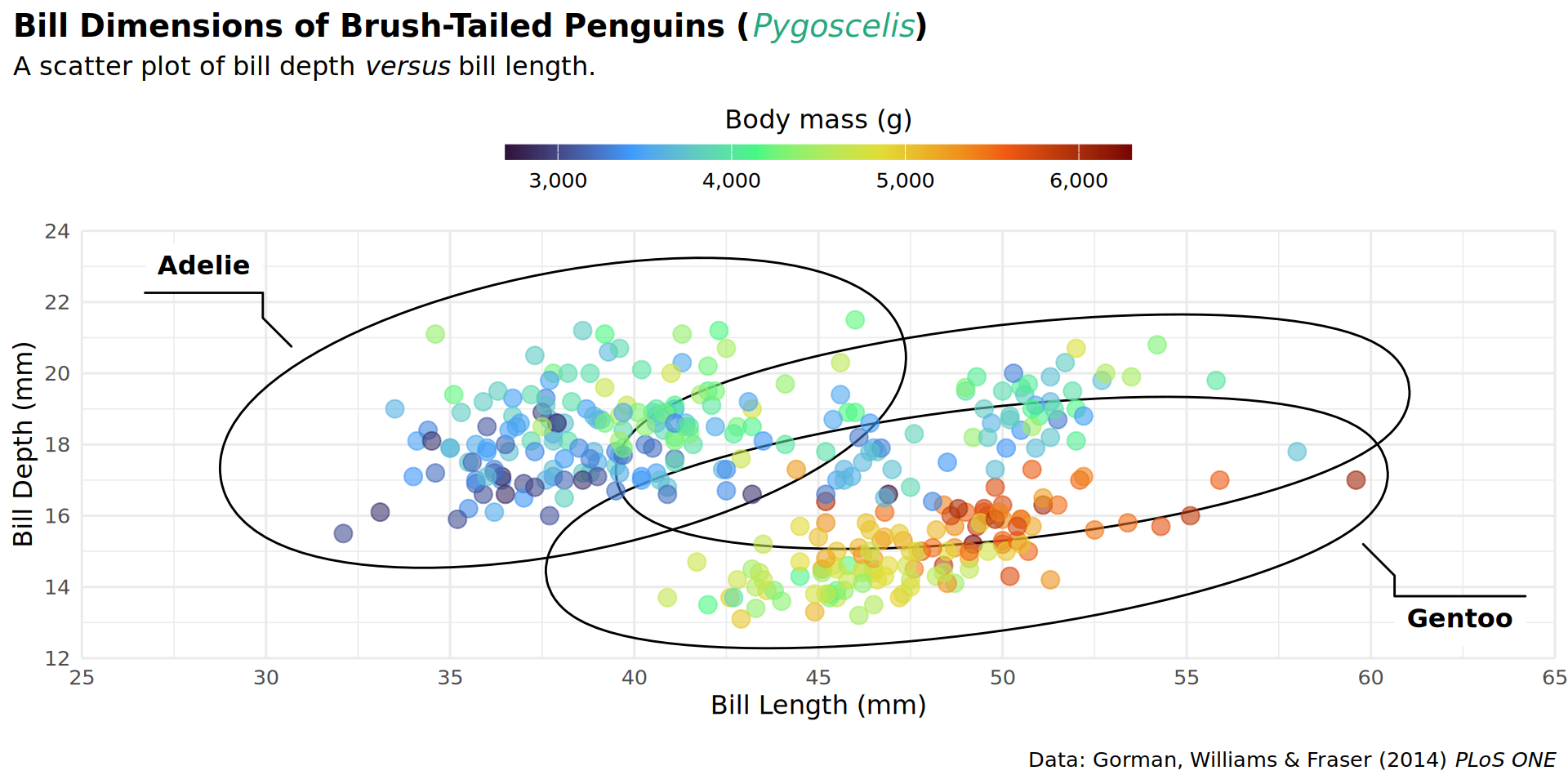
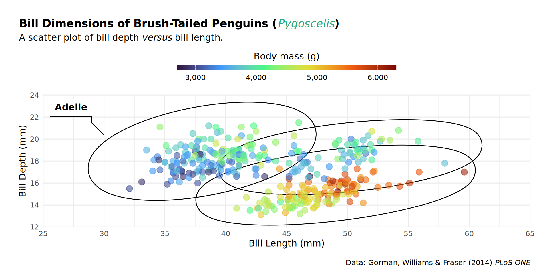
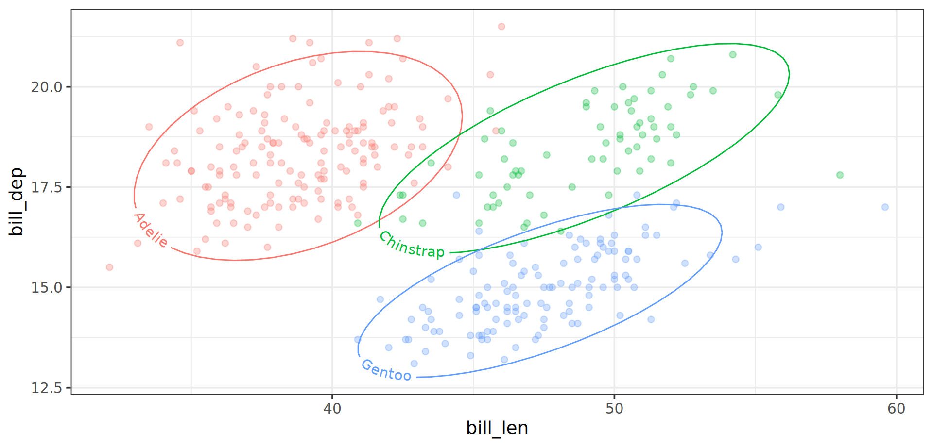
ggplot(aes(x = bill_len, y = bill_dep)) +
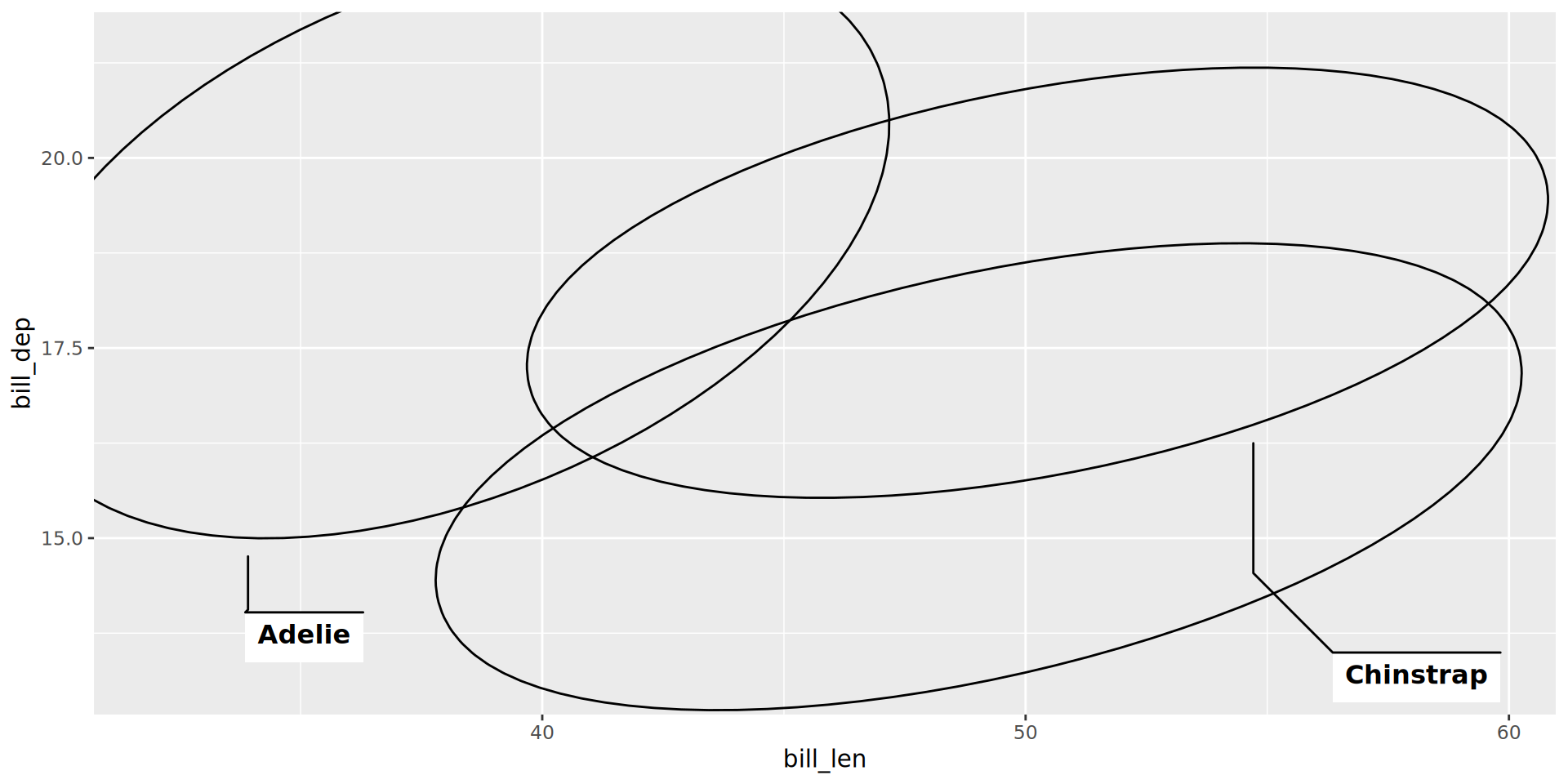
ggforce::geom_mark_ellipse(
aes(fill = species, label = species), alpha = 0,
show.legend = FALSE
) +
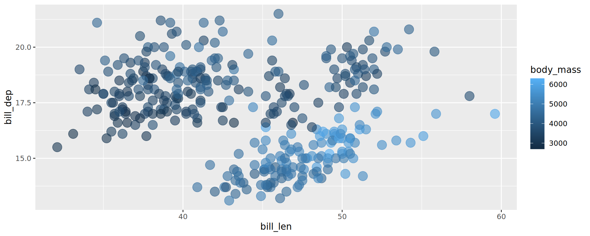
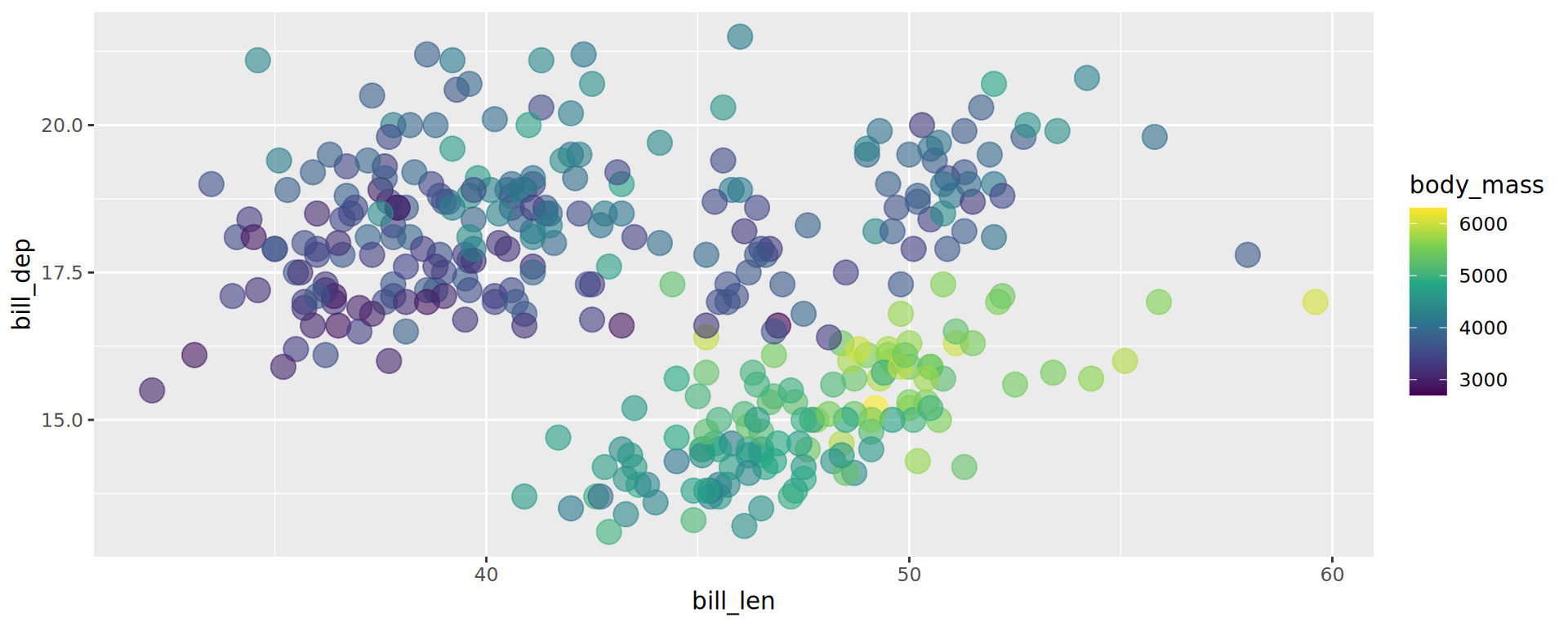
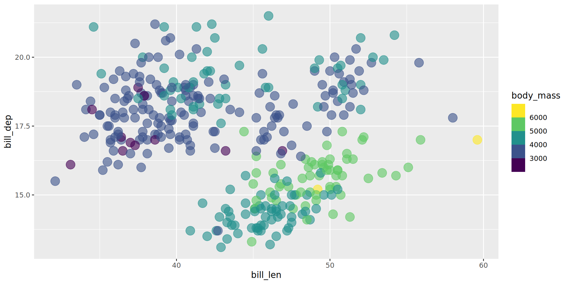
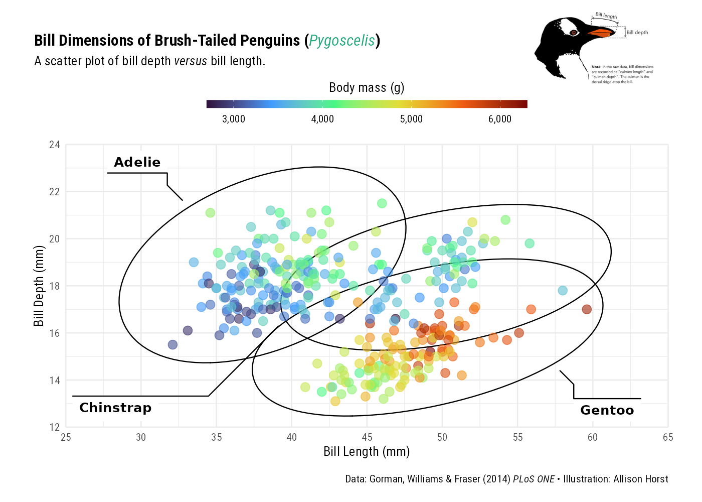
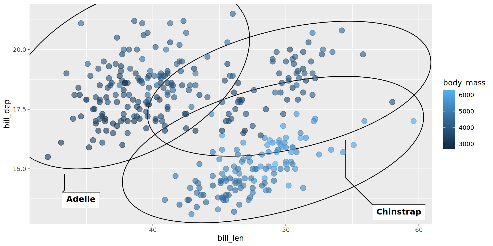
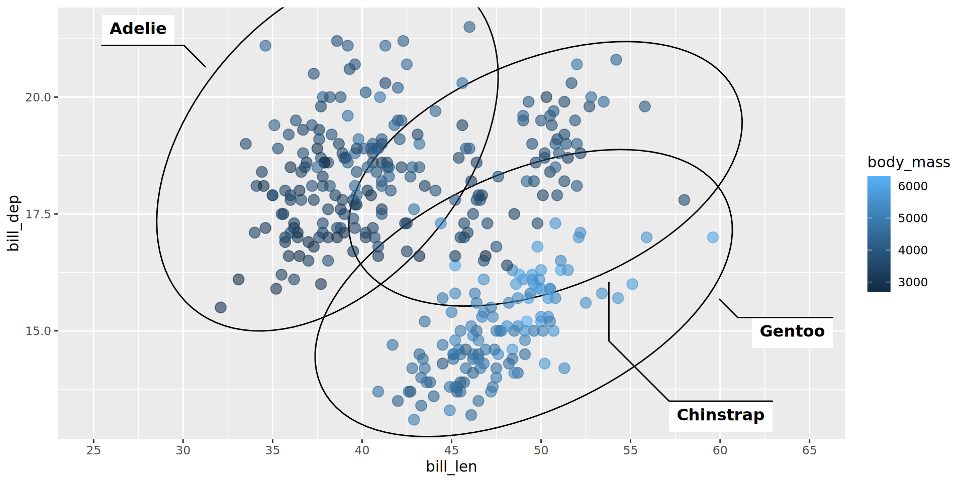
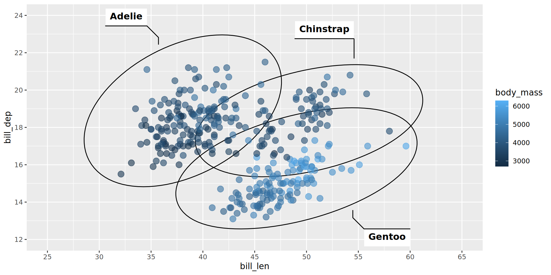
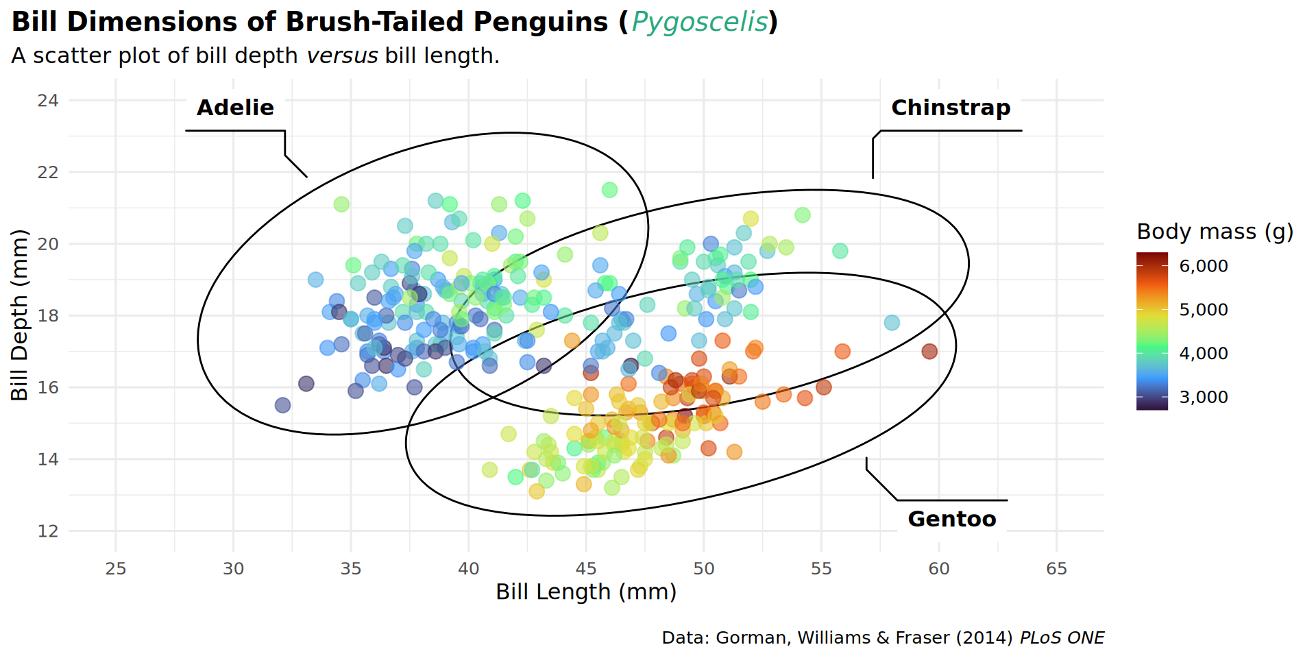
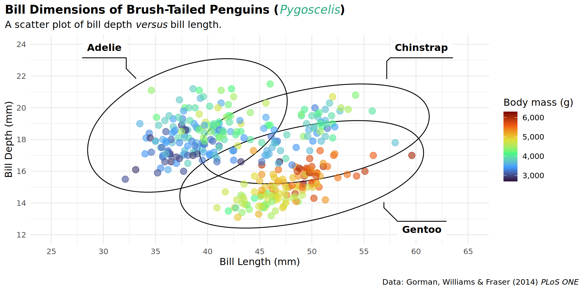
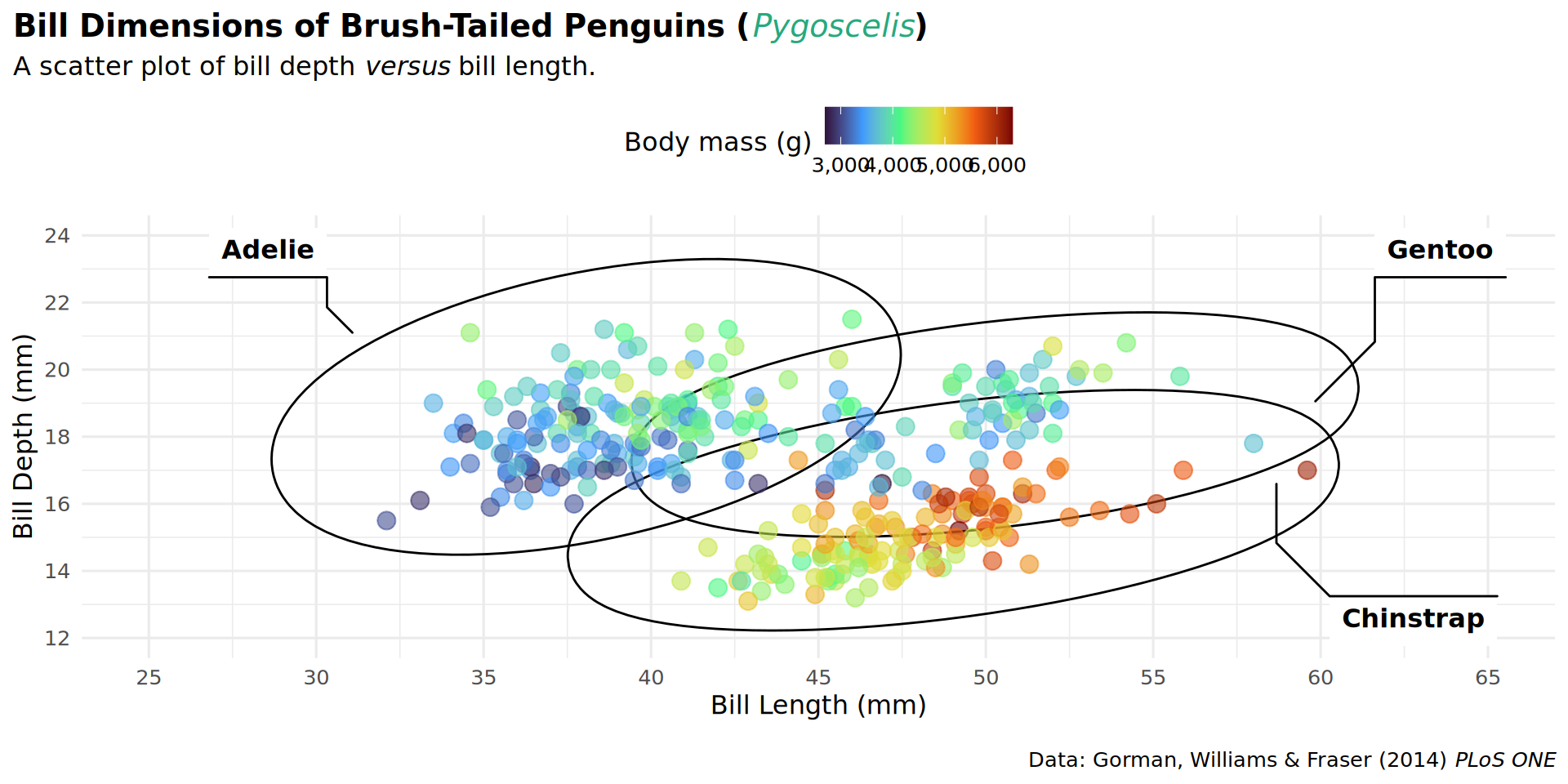
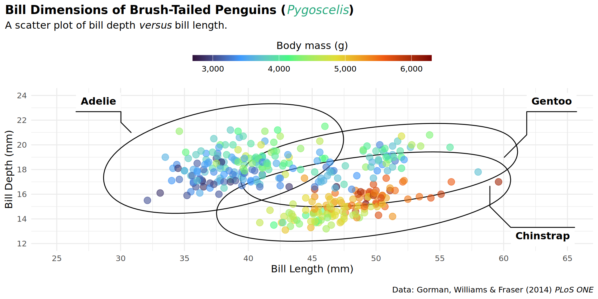
geom_point(aes(color = body_mass), alpha = .6, size = 3.5) +
scale_x_continuous(breaks = seq(25, 65, by = 5), limits = c(25, 65)) +
scale_y_continuous(breaks = seq(12, 24, by = 2), limits = c(12, 24)) +
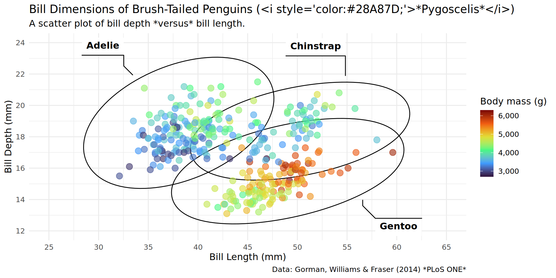
scale_color_viridis_c(option = "turbo", labels = scales::comma) +
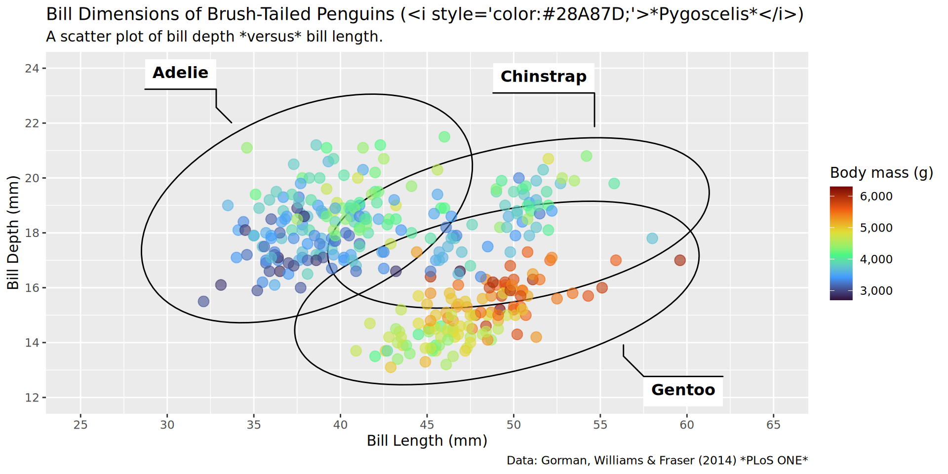
labs(
title = "Bill Dimensions of Brush-Tailed Penguins (<i style='color:#28A87D;'>*Pygoscelis*</i>)",
subtitle = 'A scatter plot of bill depth *versus* bill length.',
caption = "Data: Gorman, Williams & Fraser (2014) *PLoS ONE*",
x = "Bill Length (mm)",
y = "Bill Depth (mm)",
color = "Body mass (g)") +
theme_minimal(base_family = "RobotoCondensed", base_size = 12) +
theme(plot.title = element_markdown(face = "bold"),
plot.subtitle = element_markdown(),
plot.caption = element_markdown(margin = margin(t = 15)),
axis.title.x = element_markdown(),
axis.title.y = element_markdown()) +
theme(plot.title.position = "plot") +
theme(plot.caption.position = "plot") +
theme(legend.position = "top") +
guides(color = guide_colorbar(title.position = "top",
title.hjust = .5,
barwidth = unit(20, "lines"),
barheight = unit(.5, "lines"))) +
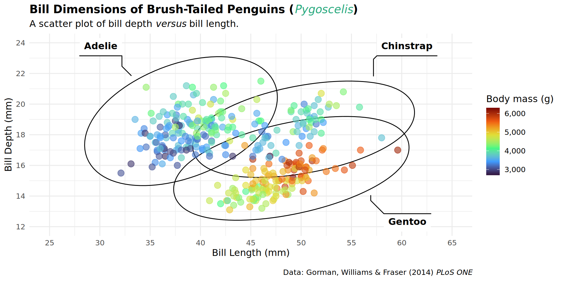
coord_cartesian(expand = FALSE, clip = "off") +
theme(plot.margin = margin(t = 25, r = 25, b = 10, l = 25)) +
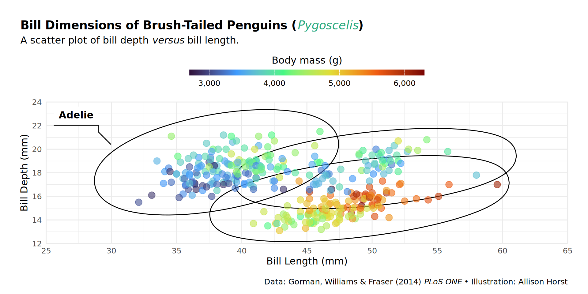
labs(caption = "Data: Gorman, Williams & Fraser (2014) *PLoS ONE* • Illustration: Allison Horst") +
patchwork::inset_element(culmen, left = 0.82, bottom = 0.83, right = 1, top = 1, align_to = 'full')