# A tibble: 6 × 2
  subject_id gender_age
       <int> <chr>
1       1001 m-56
2       1002 f-22
3       1003 m-36
4       1004 f-30
5       1005 m-64
6 1006 f-41 Principles of tidy data
and tidyr
Aurélien Ginolhac, DHML
University of Luxembourg
Tuesday 24 March, 2026
Learning objectives
You will learn to:

- List the principles of tidy data to structure data in tables
- Identify errors in existing data sets
- Rearrangements
- Split columns
- Unite columns
- Pivot to long format
- Pivot to wider
Credit: Artwork by Allison Horst
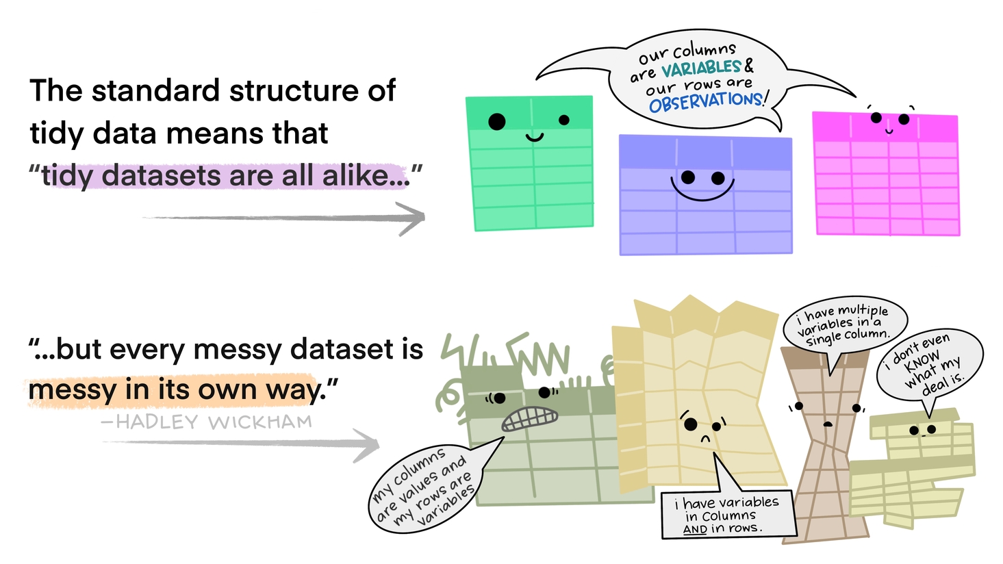
A definition of tidy data
- Variable: A quantity, quality, or property that you can measure.
- Observation: A set of values that display the relationship between variables. To be an observation, values need to be measured under similar conditions, usually measured on the same observational unit at the same time.
- Value: The state of a variable that you observe when you measure it.
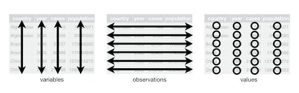
- Each variable forms a column.
- Each observation forms a row.
- Each type of observational unit forms a table.
Source: Garret Grolemund and vignette("tidy-data")
Bad data exercise
Questions
- The following table lists data from two questionnaires –stai and rec– recorded in different languages.
- What’s wrong with the Excel sheet?
- Which problems are tidy issues?

Tidy errors
| Error | Tidy violation | Comment |
|---|---|---|
| Person name | No | Data protection violation |
| Identical column names | Yes | Variable error |
| Inconsistent variables names | No | Bad practice |
| Non-English columns names | No | Bad practice |
| Color coding | No | The horror, the horror |
| Inconsistent dates | No | Use ISO8601 |
| Multiple columns for one item | Yes | One observation per line |
| Redundant information | Yes | Each variable is in its own column |
| Repeated rows | Yes | Each observation is in its own row |
| Missing coding | Yes/No | Each value in its own cell |
| Unnecessary information (Birthdate, comments) | No | Bad practice |
| Name of the table | No | Bad practice |
Basic rearrangements
tidyr
Splitting values into columns
Key-value pairs
Collating columns into one
Input tibble
Unite columns into one
# A tibble: 3 × 2
  date       value
  <chr>      <chr>
1 2015-11-23 high
2 2014-2-1   low
3 2014-4-30  low
No need to clean up old columns.
Parsing dates
A gift from your collaborators
# A tibble: 5 × 2
  subject visit_date
    <dbl> <chr>
1       1 01/07/2001
2       2 01.MAY.2012
3       3 12-07-2015
4       4 4/5/14
5       5 12. Jun 1999
Mix of everything
lubridate to the rescue!
# A tibble: 5 × 3
  subject visit_date   good_date
    <dbl> <chr>        <date>
1       1 01/07/2001   2001-07-01
2       2 01.MAY.2012  2012-05-01
3       3 12-07-2015   2015-07-12
4       4 4/5/14       2014-05-04
5       5 12. Jun 1999 1999-06-12
lubridate has a range of functions for parsing ill-formatted dates and times.
Separate rows with multiple entries
Multiple values per cell
# A tibble: 3 × 3
  subject_id visit_id measured
       <int> <chr>    <chr>
1       1001 1,2, 3   9,0, 11
2       1002 1|2      11, 3
3       1003 1        12
Note the incoherent white space and separators.
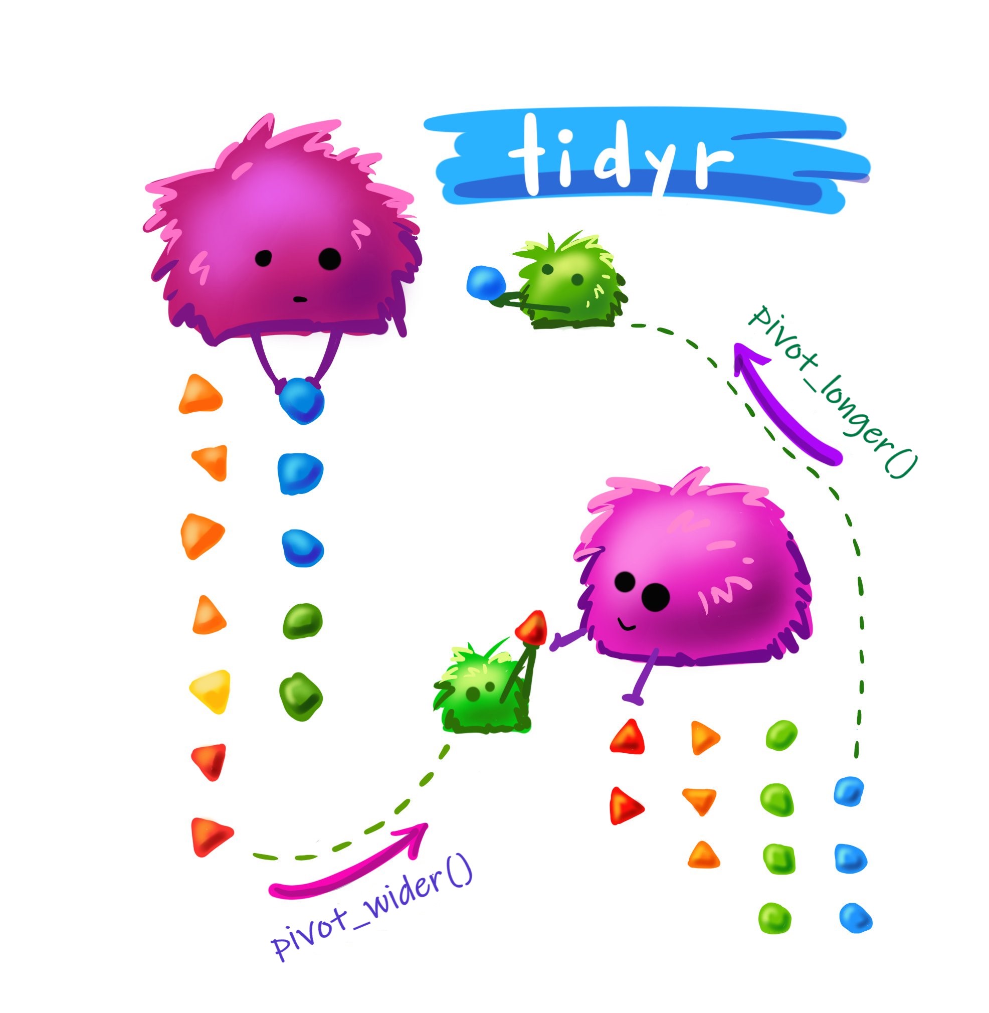
Pivot, each variable in its own column
Chromosome lengths
Is it in tidy format?
Pivot to the longer format
Act on all columns but org
# A tibble: 6 × 3
  org   chromosome length_bp
  <chr> <chr>          <dbl>
1 yeast chr1          230218
2 yeast chr2          813184
3 yeast MT             85779
4 mouse chr1       195154279
5 mouse chr2       181755017
6 mouse MT             16299
The org IDs are replicated by the number of pivoted columns (3)
Pivot longer is also called melt
Pivot wider, useful for some computation
Compute the absolute difference
Of chromosome lengths between mouse and yeast?
Hint
We need the org in their own column
# A tibble: 6 × 3
  org   chromosome length_bp
  <chr> <chr>          <dbl>
1 yeast chr1          230218
2 yeast chr2          813184
3 yeast MT             85779
4 mouse chr1       195154279
5 mouse chr2       181755017
6 mouse MT             16299
Pivot wider, ids are now chromosomes
# A tibble: 3 × 3
  chromosome  yeast     mouse
  <chr>       <dbl>     <dbl>
1 chr1       230218 195154279
2 chr2       813184 181755017
3 MT          85779     16299
Now do the absolute diff
Longer vs Wider
Credit: Artwork by Allison Horst
Before we stop
You learned to:
- What is the tidy format
- Split and Unite columns
- Pivot long / wide
Further reading 📚
- Rectangling Taming data into rectangles
Acknowledgments 🙏 👏
- Hadley Wickham
- Roland Krause
- Alison Hill
- Artwork by Allison Horst
Thank you for your attention!

![]()