Data wrangling
dplyr
Aurélien Ginolhac
University of Luxembourg
Tuesday 14 April, 2026
Learning objectives
![]()
You will learn to:
 Data munging
- Preparing data is the most time consuming part of data analysis.
- Individual steps might look easy.
- Essential part of understanding the data you’re working with.
- Additional data preparation before modeling is impossible to avoid.
dplyr is a tool box for working with data in tibbles, offering a unified language for operations scattered through base .
Key operations
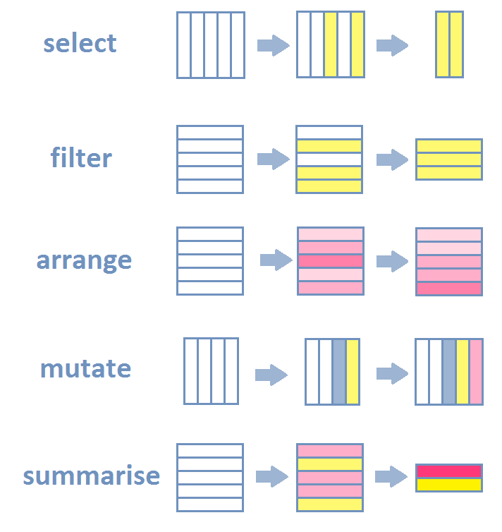
Source: Lise Vaudor
Data wrangling learning
Organisation
Split into 3 slide decks (1, 2, 3)
- Learn the grammar to operate on rows and columns of a table
- Selection and manipulation of (1)
- Observations,
- Variables and
- Values
- Grouping and summarizing (2)
- Joining and intersecting tibbles (3)
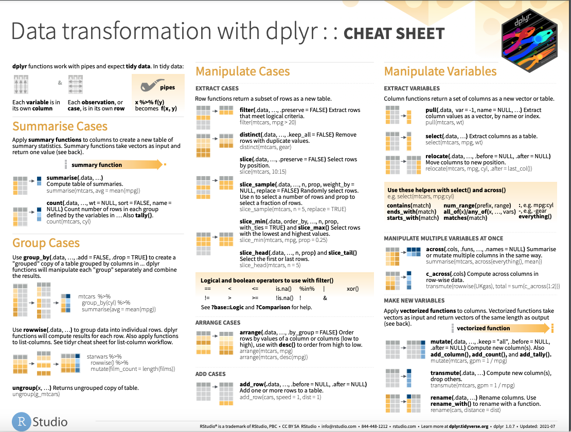
dplyr introduction: Cheatsheet
Companion real data for this course
Description
Van’t Veer & Sleegers. (2019) Psychology data from an exploration of the effect of anticipatory stress on disgust vs. non-disgust related moral judgments. J. of Open Psychology Data.
Data is (largely) tidy.
Typical data you might see in the wild.
Moral dilemma (trolley problem, survival after plane crash, etc.
moral)Standard questionnaires
- Private Body Consciousness (
PBC, range 0 - 4, as the awareness of internal sensations) - Rational-Experiential Inventory (
REI, range 1 - 5, assesses tendencies to engage in rational and experiential information processing) - Multidimensional Assessment of Interoceptive Awareness (
MAIA, range 0 - 5, feeling the feels) - State Trait Anxiety Inventory (
STAI, feelings such as apprehension, tension, nervousness, and worry)
- Private Body Consciousness (
Your turn!
Load the data into your RStudio session if you wish to follow along
# A tibble: 188 × 158
   start_date end_date  finished condition subject gender   age mood_pre
   <chr>      <chr>        <dbl> <chr>       <dbl> <chr>  <dbl>    <dbl>
 1 11/3/2014  11/3/2014        1 control         2 female    24       81
 2 11/3/2014  11/3/2014        1 stress          1 female    19       59
 3 11/3/2014  11/3/2014        1 stress          3 female    19       22
 4 11/3/2014  11/3/2014        1 stress          4 female    22       53
 5 11/3/2014  11/3/2014        1 control         7 female    22       48
 6 11/3/2014  11/3/2014        1 stress          6 female    22       73
 7 11/3/2014  11/3/2014        1 control         5 female    18       NA
 8 11/3/2014  11/3/2014        1 control         9 male      20      100
 9 11/3/2014  11/3/2014        1 stress         16 female    21       67
10 11/3/2014  11/3/2014        1 stress         13 female    19       30
# ℹ 178 more rows
# ℹ 150 more variables: mood_post <dbl>, STAI_pre_1_1 <dbl>,
#   STAI_pre_1_2 <dbl>, STAI_pre_1_3 <dbl>, STAI_pre_1_4 <dbl>,
#   STAI_pre_1_5 <dbl>, STAI_pre_1_6 <dbl>, STAI_pre_1_7 <dbl>,
#   STAI_pre_2_1 <dbl>, STAI_pre_2_2 <dbl>, STAI_pre_2_3 <dbl>,
#   STAI_pre_2_4 <dbl>, STAI_pre_2_5 <dbl>, STAI_pre_2_6 <dbl>,
#   STAI_pre_2_7 <dbl>, STAI_pre_3_1 <dbl>, STAI_pre_3_2 <dbl>, …
Selecting columns
The columns you want: select(tibble, col1, ...)
# A tibble: 188 × 3
   gender   age condition
   <chr>  <dbl> <chr>
 1 female    24 control
 2 female    19 stress
 3 female    19 stress
 4 female    22 stress
 5 female    22 control
 6 female    22 stress
 7 female    18 control
 8 male      20 control
 9 female    21 stress
10 female    19 stress
# ℹ 178 more rows
Also in the order chosen
tidyselect
Helper functions
To select columns with names that:
contains()- a stringstarts_with()- a stringends_with()- a stringone_of()- names in a character vectormatches()- using regular expressionseverything()- all remaining columnslast_col()- last column
Danger
Avoid selecting columns by index!
To ensure reproducibility select columns by bare names
# A tibble: 188 × 10
   moral_dilemma_dog moral_dilemma_wallet moral_dilemma_plane
               <dbl>                <dbl>               <dbl>
 1                 9                    9                   8
 2                 9                    9                   9
 3                 8                    7                   8
 4                 8                    4                   8
 5                 3                    9                   9
 6                 9                    9                   9
 7                 9                    5                   7
 8                 9                    4                   1
 9                 6                    9                   3
10                 6                    8                   9
# ℹ 178 more rows
# ℹ 7 more variables: moral_dilemma_resume <dbl>, moral_dilemma_kitten <dbl>,
#   moral_dilemma_trolley <dbl>, moral_dilemma_control <dbl>,
#   moral_judgment <dbl>, moral_judgment_disgust <dbl>,
#   moral_judgment_non_disgust <dbl>
Combining helpers
Remark
- Found in several functions (
x)read_delim(... col_select = x)mutate(..., .by = x)summarise(..., .by = x)pivot_longer(..., .cols = x)nest(..., .by = x)across()
- Helpers are evaluated from left to right, it matters for negative selection!
# A tibble: 3 × 9
  start_date end_date moral_dilemma_dog moral_dilemma_wallet moral_dilemma_plane
  <chr>      <chr>                <dbl>                <dbl>               <dbl>
1 11/3/2014  11/3/20…                 9                    9                   8
2 11/3/2014  11/3/20…                 9                    9                   9
3 11/3/2014  11/3/20…                 8                    7                   8
# ℹ 4 more variables: moral_dilemma_resume <dbl>, moral_dilemma_kitten <dbl>,
# moral_dilemma_trolley <dbl>, moral_dilemma_control <dbl># A tibble: 3 × 157
finished condition subject gender age mood_pre mood_post STAI_pre_1_1
<dbl> <chr> <dbl> <chr> <dbl> <dbl> <dbl> <dbl>
1 1 control 2 female 24 81 NA 2
2 1 stress 1 female 19 59 42 3
3 1 stress 3 female 19 22 60 4
# ℹ 149 more variables: STAI_pre_1_2 <dbl>, STAI_pre_1_3 <dbl>,
# STAI_pre_1_4 <dbl>, STAI_pre_1_5 <dbl>, STAI_pre_1_6 <dbl>,
# STAI_pre_1_7 <dbl>, STAI_pre_2_1 <dbl>, STAI_pre_2_2 <dbl>,
# STAI_pre_2_3 <dbl>, STAI_pre_2_4 <dbl>, STAI_pre_2_5 <dbl>,
# STAI_pre_2_6 <dbl>, STAI_pre_2_7 <dbl>, STAI_pre_3_1 <dbl>,
# STAI_pre_3_2 <dbl>, STAI_pre_3_3 <dbl>, STAI_pre_3_4 <dbl>,
# STAI_pre_3_5 <dbl>, STAI_pre_3_6 <dbl>, STAI_post_1_1 <dbl>, …Column start_date is gone with the first helper
Filtering for rows: filter()
Let’s take a look at all the data that were excluded.
# A tibble: 3 × 158
  start_date end_date finished condition subject gender   age mood_pre mood_post
  <chr>      <chr>       <dbl> <chr>       <dbl> <chr>  <dbl>    <dbl>     <dbl>
1 11/3/2014  11/3/20…        1 stress         28 male      22       53        68
2 11/3/2014  11/3/20…        1 stress         32 female    19       74        77
3 11/7/2014  11/7/20…        1 stress        181 male      22       47        65
# ℹ 149 more variables: STAI_pre_1_1 <dbl>, STAI_pre_1_2 <dbl>,
#   STAI_pre_1_3 <dbl>, STAI_pre_1_4 <dbl>, STAI_pre_1_5 <dbl>,
#   STAI_pre_1_6 <dbl>, STAI_pre_1_7 <dbl>, STAI_pre_2_1 <dbl>,
#   STAI_pre_2_2 <dbl>, STAI_pre_2_3 <dbl>, STAI_pre_2_4 <dbl>,
#   STAI_pre_2_5 <dbl>, STAI_pre_2_6 <dbl>, STAI_pre_2_7 <dbl>,
#   STAI_pre_3_1 <dbl>, STAI_pre_3_2 <dbl>, STAI_pre_3_3 <dbl>,
# STAI_pre_3_4 <dbl>, STAI_pre_3_5 <dbl>, STAI_pre_3_6 <dbl>, …- Test equality sign is
== =is an assignment.
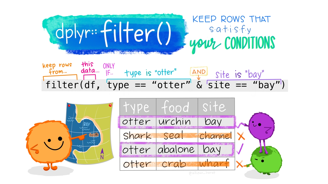
Artwork by @allison_horst
Filtering rows
Multiple conditions: AND
- comma separated conditions are equivalent to
&(AND). - Filter for females older than 20.
# A tibble: 34 × 158
   start_date end_date  finished condition subject gender   age mood_pre
   <chr>      <chr>        <dbl> <chr>       <dbl> <chr>  <dbl>    <dbl>
 1 11/3/2014  11/3/2014        1 control         2 female    24       81
 2 11/3/2014  11/3/2014        1 stress          4 female    22       53
 3 11/3/2014  11/3/2014        1 control         7 female    22       48
 4 11/3/2014  11/3/2014        1 stress          6 female    22       73
 5 11/3/2014  11/3/2014        1 stress         16 female    21       67
 6 11/3/2014  11/3/2014        1 control        10 female    21       72
 7 11/3/2014  11/3/2014        1 control        23 female    23       78
 8 11/3/2014  11/3/2014        1 control        29 female    22       65
 9 11/3/2014  11/3/2014        1 stress         36 female    21       32
10 11/3/2014  11/3/2014        1 control        31 female    23       69
# ℹ 24 more rows
# ℹ 150 more variables: mood_post <dbl>, STAI_pre_1_1 <dbl>,
#   STAI_pre_1_2 <dbl>, STAI_pre_1_3 <dbl>, STAI_pre_1_4 <dbl>,
#   STAI_pre_1_5 <dbl>, STAI_pre_1_6 <dbl>, STAI_pre_1_7 <dbl>,
#   STAI_pre_2_1 <dbl>, STAI_pre_2_2 <dbl>, STAI_pre_2_3 <dbl>,
#   STAI_pre_2_4 <dbl>, STAI_pre_2_5 <dbl>, STAI_pre_2_6 <dbl>,
#   STAI_pre_2_7 <dbl>, STAI_pre_3_1 <dbl>, STAI_pre_3_2 <dbl>, …
Multiple conditions: OR
- vertical bar (
|) separated conditions are combined with OR. - Filter females or age > 20 (so males too)
# A tibble: 164 × 158
   start_date end_date  finished condition subject gender   age mood_pre
   <chr>      <chr>        <dbl> <chr>       <dbl> <chr>  <dbl>    <dbl>
 1 11/3/2014  11/3/2014        1 control         2 female    24       81
 2 11/3/2014  11/3/2014        1 stress          1 female    19       59
 3 11/3/2014  11/3/2014        1 stress          3 female    19       22
 4 11/3/2014  11/3/2014        1 stress          4 female    22       53
 5 11/3/2014  11/3/2014        1 control         7 female    22       48
 6 11/3/2014  11/3/2014        1 stress          6 female    22       73
 7 11/3/2014  11/3/2014        1 control         5 female    18       NA
 8 11/3/2014  11/3/2014        1 stress         16 female    21       67
 9 11/3/2014  11/3/2014        1 stress         13 female    19       30
10 11/3/2014  11/3/2014        1 stress         18 female    19       55
# ℹ 154 more rows
# ℹ 150 more variables: mood_post <dbl>, STAI_pre_1_1 <dbl>,
#   STAI_pre_1_2 <dbl>, STAI_pre_1_3 <dbl>, STAI_pre_1_4 <dbl>,
#   STAI_pre_1_5 <dbl>, STAI_pre_1_6 <dbl>, STAI_pre_1_7 <dbl>,
#   STAI_pre_2_1 <dbl>, STAI_pre_2_2 <dbl>, STAI_pre_2_3 <dbl>,
#   STAI_pre_2_4 <dbl>, STAI_pre_2_5 <dbl>, STAI_pre_2_6 <dbl>,
#   STAI_pre_2_7 <dbl>, STAI_pre_3_1 <dbl>, STAI_pre_3_2 <dbl>, …
Filtering out rows
Row vs column selection
filter()acts on rowsselect()acts on columns
- Remove excluded participants (initially 188 rows)
- Combine with
relocate()to placemoodcolumns first
# A tibble: 185 × 158
   mood_pre mood_post start_date end_date  finished condition subject gender
      <dbl>     <dbl> <chr>      <chr>        <dbl> <chr>       <dbl> <chr>
 1       81        NA 11/3/2014  11/3/2014        1 control         2 female
 2       59        42 11/3/2014  11/3/2014        1 stress          1 female
 3       22        60 11/3/2014  11/3/2014        1 stress          3 female
 4       53        68 11/3/2014  11/3/2014        1 stress          4 female
 5       48        NA 11/3/2014  11/3/2014        1 control         7 female
 6       73        73 11/3/2014  11/3/2014        1 stress          6 female
 7       NA        NA 11/3/2014  11/3/2014        1 control         5 female
 8      100        NA 11/3/2014  11/3/2014        1 control         9 male
 9       67        74 11/3/2014  11/3/2014        1 stress         16 female
10       30        68 11/3/2014  11/3/2014        1 stress         13 female
# ℹ 175 more rows
# ℹ 150 more variables: age <dbl>, STAI_pre_1_1 <dbl>, STAI_pre_1_2 <dbl>,
#   STAI_pre_1_3 <dbl>, STAI_pre_1_4 <dbl>, STAI_pre_1_5 <dbl>,
#   STAI_pre_1_6 <dbl>, STAI_pre_1_7 <dbl>, STAI_pre_2_1 <dbl>,
#   STAI_pre_2_2 <dbl>, STAI_pre_2_3 <dbl>, STAI_pre_2_4 <dbl>,
#   STAI_pre_2_5 <dbl>, STAI_pre_2_6 <dbl>, STAI_pre_2_7 <dbl>,
#   STAI_pre_3_1 <dbl>, STAI_pre_3_2 <dbl>, STAI_pre_3_3 <dbl>, …
Set operations with filter()
- For larger operations use filtering joins such as
semi_join(). - Below,
tidyselecthelper:for a range of columns
# A tibble: 79 × 7
   start_date end_date  finished condition subject gender   age
   <chr>      <chr>        <dbl> <chr>       <dbl> <chr>  <dbl>
 1 11/3/2014  11/3/2014        1 control         2 female    24
 2 11/3/2014  11/3/2014        1 stress          1 female    19
 3 11/3/2014  11/3/2014        1 stress          3 female    19
 4 11/3/2014  11/3/2014        1 stress          4 female    22
 5 11/3/2014  11/3/2014        1 control         7 female    22
 6 11/3/2014  11/3/2014        1 stress          6 female    22
 7 11/3/2014  11/3/2014        1 control         5 female    18
 8 11/3/2014  11/3/2014        1 control         9 male      20
 9 11/3/2014  11/3/2014        1 stress         16 female    21
10 11/3/2014  11/3/2014        1 stress         13 female    19
# ℹ 69 more rows# A tibble: 79 × 7
start_date end_date finished condition subject gender age
<chr> <chr> <dbl> <chr> <dbl> <chr> <dbl>
1 11/3/2014 11/3/2014 1 control 2 female 24
2 11/3/2014 11/3/2014 1 stress 1 female 19
3 11/3/2014 11/3/2014 1 stress 3 female 19
4 11/3/2014 11/3/2014 1 stress 4 female 22
5 11/3/2014 11/3/2014 1 control 7 female 22
6 11/3/2014 11/3/2014 1 stress 6 female 22
7 11/3/2014 11/3/2014 1 control 5 female 18
8 11/3/2014 11/3/2014 1 control 9 male 20
9 11/3/2014 11/3/2014 1 stress 16 female 21
10 11/3/2014 11/3/2014 1 stress 13 female 19
# ℹ 69 more rows%in% is an important operator in
Filter out rows that are unique: distinct()
Do we have different start / end dates?
# A tibble: 188 × 2
   start_date end_date
   <chr>      <chr>
 1 11/3/2014  11/3/2014
 2 11/3/2014  11/3/2014
 3 11/3/2014  11/3/2014
 4 11/3/2014  11/3/2014
 5 11/3/2014  11/3/2014
 6 11/3/2014  11/3/2014
 7 11/3/2014  11/3/2014
 8 11/3/2014  11/3/2014
 9 11/3/2014  11/3/2014
10 11/3/2014  11/3/2014
# ℹ 178 more rows
Too many identical rows.
Use distinct() to remove duplicated rows:
# A tibble: 5 × 2
  start_date end_date
  <chr>      <chr>
1 11/3/2014  11/3/2014
2 11/4/2014  11/4/2014
3 11/5/2014  11/5/2014
4 11/6/2014  11/6/2014
5 11/7/2014 11/7/2014- Also possible (except columns order):
Filter out observations (>= v1.2.0)
Filter out rows from columns with NA can be tricky. Filter out male with mood_post > 30
# A tibble: 147 × 158
   start_date end_date  finished condition subject gender   age mood_pre
   <chr>      <chr>        <dbl> <chr>       <dbl> <chr>  <dbl>    <dbl>
 1 11/3/2014  11/3/2014        1 control         2 female    24       81
 2 11/3/2014  11/3/2014        1 stress          1 female    19       59
 3 11/3/2014  11/3/2014        1 stress          3 female    19       22
 4 11/3/2014  11/3/2014        1 stress          4 female    22       53
 5 11/3/2014  11/3/2014        1 control         7 female    22       48
 6 11/3/2014  11/3/2014        1 stress          6 female    22       73
 7 11/3/2014  11/3/2014        1 control         5 female    18       NA
 8 11/3/2014  11/3/2014        1 stress         16 female    21       67
 9 11/3/2014  11/3/2014        1 stress         13 female    19       30
10 11/3/2014  11/3/2014        1 stress         18 female    19       55
# ℹ 137 more rows
# ℹ 150 more variables: mood_post <dbl>, STAI_pre_1_1 <dbl>,
#   STAI_pre_1_2 <dbl>, STAI_pre_1_3 <dbl>, STAI_pre_1_4 <dbl>,
#   STAI_pre_1_5 <dbl>, STAI_pre_1_6 <dbl>, STAI_pre_1_7 <dbl>,
#   STAI_pre_2_1 <dbl>, STAI_pre_2_2 <dbl>, STAI_pre_2_3 <dbl>,
#   STAI_pre_2_4 <dbl>, STAI_pre_2_5 <dbl>, STAI_pre_2_6 <dbl>,
#   STAI_pre_2_7 <dbl>, STAI_pre_3_1 <dbl>, STAI_pre_3_2 <dbl>, …
Seems correct but it’s not
We removed males with missing date in mood_post, while we shouldn’t.
# A tibble: 173 × 158
   start_date end_date  finished condition subject gender   age mood_pre
   <chr>      <chr>        <dbl> <chr>       <dbl> <chr>  <dbl>    <dbl>
 1 11/3/2014  11/3/2014        1 control         2 female    24       81
 2 11/3/2014  11/3/2014        1 stress          1 female    19       59
 3 11/3/2014  11/3/2014        1 stress          3 female    19       22
 4 11/3/2014  11/3/2014        1 stress          4 female    22       53
 5 11/3/2014  11/3/2014        1 control         7 female    22       48
 6 11/3/2014  11/3/2014        1 stress          6 female    22       73
 7 11/3/2014  11/3/2014        1 control         5 female    18       NA
 8 11/3/2014  11/3/2014        1 control         9 male      20      100
 9 11/3/2014  11/3/2014        1 stress         16 female    21       67
10 11/3/2014  11/3/2014        1 stress         13 female    19       30
# ℹ 163 more rows
# ℹ 150 more variables: mood_post <dbl>, STAI_pre_1_1 <dbl>,
#   STAI_pre_1_2 <dbl>, STAI_pre_1_3 <dbl>, STAI_pre_1_4 <dbl>,
#   STAI_pre_1_5 <dbl>, STAI_pre_1_6 <dbl>, STAI_pre_1_7 <dbl>,
#   STAI_pre_2_1 <dbl>, STAI_pre_2_2 <dbl>, STAI_pre_2_3 <dbl>,
#   STAI_pre_2_4 <dbl>, STAI_pre_2_5 <dbl>, STAI_pre_2_6 <dbl>,
#   STAI_pre_2_7 <dbl>, STAI_pre_3_1 <dbl>, STAI_pre_3_2 <dbl>, …
Actual correct filter():
# A tibble: 173 × 158
   start_date end_date  finished condition subject gender   age mood_pre
   <chr>      <chr>        <dbl> <chr>       <dbl> <chr>  <dbl>    <dbl>
 1 11/3/2014  11/3/2014        1 control         2 female    24       81
 2 11/3/2014  11/3/2014        1 stress          1 female    19       59
 3 11/3/2014  11/3/2014        1 stress          3 female    19       22
 4 11/3/2014  11/3/2014        1 stress          4 female    22       53
 5 11/3/2014  11/3/2014        1 control         7 female    22       48
 6 11/3/2014  11/3/2014        1 stress          6 female    22       73
 7 11/3/2014  11/3/2014        1 control         5 female    18       NA
 8 11/3/2014  11/3/2014        1 control         9 male      20      100
 9 11/3/2014  11/3/2014        1 stress         16 female    21       67
10 11/3/2014  11/3/2014        1 stress         13 female    19       30
# ℹ 163 more rows
# ℹ 150 more variables: mood_post <dbl>, STAI_pre_1_1 <dbl>,
#   STAI_pre_1_2 <dbl>, STAI_pre_1_3 <dbl>, STAI_pre_1_4 <dbl>,
#   STAI_pre_1_5 <dbl>, STAI_pre_1_6 <dbl>, STAI_pre_1_7 <dbl>,
#   STAI_pre_2_1 <dbl>, STAI_pre_2_2 <dbl>, STAI_pre_2_3 <dbl>,
#   STAI_pre_2_4 <dbl>, STAI_pre_2_5 <dbl>, STAI_pre_2_6 <dbl>,
#   STAI_pre_2_7 <dbl>, STAI_pre_3_1 <dbl>, STAI_pre_3_2 <dbl>, …
Combining condition helpers (>= v1.2.0)
You noticed we cannot use a comma for AND in complex expressions.
# A tibble: 173 × 158
   start_date end_date  finished condition subject gender   age mood_pre
   <chr>      <chr>        <dbl> <chr>       <dbl> <chr>  <dbl>    <dbl>
 1 11/3/2014  11/3/2014        1 control         2 female    24       81
 2 11/3/2014  11/3/2014        1 stress          1 female    19       59
 3 11/3/2014  11/3/2014        1 stress          3 female    19       22
 4 11/3/2014  11/3/2014        1 stress          4 female    22       53
 5 11/3/2014  11/3/2014        1 control         7 female    22       48
 6 11/3/2014  11/3/2014        1 stress          6 female    22       73
 7 11/3/2014  11/3/2014        1 control         5 female    18       NA
 8 11/3/2014  11/3/2014        1 control         9 male      20      100
 9 11/3/2014  11/3/2014        1 stress         16 female    21       67
10 11/3/2014  11/3/2014        1 stress         13 female    19       30
# ℹ 163 more rows
# ℹ 150 more variables: mood_post <dbl>, STAI_pre_1_1 <dbl>,
#   STAI_pre_1_2 <dbl>, STAI_pre_1_3 <dbl>, STAI_pre_1_4 <dbl>,
#   STAI_pre_1_5 <dbl>, STAI_pre_1_6 <dbl>, STAI_pre_1_7 <dbl>,
#   STAI_pre_2_1 <dbl>, STAI_pre_2_2 <dbl>, STAI_pre_2_3 <dbl>,
#   STAI_pre_2_4 <dbl>, STAI_pre_2_5 <dbl>, STAI_pre_2_6 <dbl>,
#   STAI_pre_2_7 <dbl>, STAI_pre_3_1 <dbl>, STAI_pre_3_2 <dbl>, …
when_any() combines expression with an OR statement
# A tibble: 73 × 158
   start_date end_date  finished condition subject gender   age mood_pre
   <chr>      <chr>        <dbl> <chr>       <dbl> <chr>  <dbl>    <dbl>
 1 11/3/2014  11/3/2014        1 control         2 female    24       81
 2 11/3/2014  11/3/2014        1 control         7 female    22       48
 3 11/3/2014  11/3/2014        1 control         5 female    18       NA
 4 11/3/2014  11/3/2014        1 control        12 female    18       67
 5 11/3/2014  11/3/2014        1 control        10 female    21       72
 6 11/3/2014  11/3/2014        1 control         8 female    19       59
 7 11/3/2014  11/3/2014        1 control        23 female    23       78
 8 11/3/2014  11/3/2014        1 control        21 female    18       68
 9 11/3/2014  11/3/2014        1 stress         24 female    20       66
10 11/3/2014  11/3/2014        1 control        29 female    22       65
# ℹ 63 more rows
# ℹ 150 more variables: mood_post <dbl>, STAI_pre_1_1 <dbl>,
#   STAI_pre_1_2 <dbl>, STAI_pre_1_3 <dbl>, STAI_pre_1_4 <dbl>,
#   STAI_pre_1_5 <dbl>, STAI_pre_1_6 <dbl>, STAI_pre_1_7 <dbl>,
#   STAI_pre_2_1 <dbl>, STAI_pre_2_2 <dbl>, STAI_pre_2_3 <dbl>,
#   STAI_pre_2_4 <dbl>, STAI_pre_2_5 <dbl>, STAI_pre_2_6 <dbl>,
#   STAI_pre_2_7 <dbl>, STAI_pre_3_1 <dbl>, STAI_pre_3_2 <dbl>, …
Sort columns: arrange()
A nested sorting example
- Sort by
mood_pre - Within each group of
mood_pre, sort bymood_post
Reverse sort columns
- Use
arrange()with the helper functiondesc() - For example, oldest participant first
Your turn!
Select all columns that refer to the STAI questionnaire.
Retrieve all subjects younger than 20 which are in the stress group. The column for the group is
condition.Arrange all observations by
STAI_preso that the subject with the lowest stress level is on top. What is the subject in question?
Solution
# A tibble: 188 × 42
   STAI_pre_1_1 STAI_pre_1_2 STAI_pre_1_3 STAI_pre_1_4 STAI_pre_1_5 STAI_pre_1_6
          <dbl>        <dbl>        <dbl>        <dbl>        <dbl>        <dbl>
 1            2            1            2            2            2            2
 2            3            2            3            1            3            2
 3            4            3            3            3            4            2
 4            2            2            2            2            3            1
 5            1            1            1            1            2            1
 6            2            2            1            1            2            1
 7            2            2            1            1            2            1
 8            1            1            1            1            1            1
 9            2            2            1            1            2            1
10            4            2            3            3            3            1
# ℹ 178 more rows
# ℹ 36 more variables: STAI_pre_1_7 <dbl>, STAI_pre_2_1 <dbl>,
#   STAI_pre_2_2 <dbl>, STAI_pre_2_3 <dbl>, STAI_pre_2_4 <dbl>,
#   STAI_pre_2_5 <dbl>, STAI_pre_2_6 <dbl>, STAI_pre_2_7 <dbl>,
#   STAI_pre_3_1 <dbl>, STAI_pre_3_2 <dbl>, STAI_pre_3_3 <dbl>,
#   STAI_pre_3_4 <dbl>, STAI_pre_3_5 <dbl>, STAI_pre_3_6 <dbl>,
# STAI_post_1_1 <dbl>, STAI_post_1_2 <dbl>, STAI_post_1_3 <dbl>, …# A tibble: 3 × 158
age condition start_date end_date finished subject gender mood_pre mood_post
<dbl> <chr> <chr> <chr> <dbl> <dbl> <chr> <dbl> <dbl>
1 19 stress 11/3/2014 11/3/20… 1 1 female 59 42
2 19 stress 11/3/2014 11/3/20… 1 3 female 22 60
3 19 stress 11/3/2014 11/3/20… 1 13 female 30 68
# ℹ 149 more variables: STAI_pre_1_1 <dbl>, STAI_pre_1_2 <dbl>,
# STAI_pre_1_3 <dbl>, STAI_pre_1_4 <dbl>, STAI_pre_1_5 <dbl>,
# STAI_pre_1_6 <dbl>, STAI_pre_1_7 <dbl>, STAI_pre_2_1 <dbl>,
# STAI_pre_2_2 <dbl>, STAI_pre_2_3 <dbl>, STAI_pre_2_4 <dbl>,
# STAI_pre_2_5 <dbl>, STAI_pre_2_6 <dbl>, STAI_pre_2_7 <dbl>,
# STAI_pre_3_1 <dbl>, STAI_pre_3_2 <dbl>, STAI_pre_3_3 <dbl>,
# STAI_pre_3_4 <dbl>, STAI_pre_3_5 <dbl>, STAI_pre_3_6 <dbl>, …# A tibble: 3 × 158
STAI_pre start_date end_date finished condition subject gender age mood_pre
<dbl> <chr> <chr> <dbl> <chr> <dbl> <chr> <dbl> <dbl>
1 20 11/6/2014 11/6/2014 1 stress 142 female 22 96
2 21 11/3/2014 11/3/2014 1 control 9 male 20 100
3 22 11/7/2014 11/7/2014 1 stress 162 male 19 77
# ℹ 149 more variables: mood_post <dbl>, STAI_pre_1_1 <dbl>,
# STAI_pre_1_2 <dbl>, STAI_pre_1_3 <dbl>, STAI_pre_1_4 <dbl>,
# STAI_pre_1_5 <dbl>, STAI_pre_1_6 <dbl>, STAI_pre_1_7 <dbl>,
# STAI_pre_2_1 <dbl>, STAI_pre_2_2 <dbl>, STAI_pre_2_3 <dbl>,
# STAI_pre_2_4 <dbl>, STAI_pre_2_5 <dbl>, STAI_pre_2_6 <dbl>,
# STAI_pre_2_7 <dbl>, STAI_pre_3_1 <dbl>, STAI_pre_3_2 <dbl>,
# STAI_pre_3_3 <dbl>, STAI_pre_3_4 <dbl>, STAI_pre_3_5 <dbl>, …Transforming columns
Changing column names
rename(data, new_name = old_name)
To remember the order of appearance, consider = as “was”.
# A tibble: 188 × 158
   start_date end_date   done condition subject sex      age mood_pre mood_post
   <chr>      <chr>     <dbl> <chr>       <dbl> <chr>  <dbl>    <dbl>     <dbl>
 1 11/3/2014  11/3/2014     1 control         2 female    24       81        NA
 2 11/3/2014  11/3/2014     1 stress          1 female    19       59        42
 3 11/3/2014  11/3/2014     1 stress          3 female    19       22        60
 4 11/3/2014  11/3/2014     1 stress          4 female    22       53        68
 5 11/3/2014  11/3/2014     1 control         7 female    22       48        NA
 6 11/3/2014  11/3/2014     1 stress          6 female    22       73        73
 7 11/3/2014  11/3/2014     1 control         5 female    18       NA        NA
 8 11/3/2014  11/3/2014     1 control         9 male      20      100        NA
 9 11/3/2014  11/3/2014     1 stress         16 female    21       67        74
10 11/3/2014  11/3/2014     1 stress         13 female    19       30        68
# ℹ 178 more rows
# ℹ 149 more variables: STAI_pre_1_1 <dbl>, STAI_pre_1_2 <dbl>,
#   STAI_pre_1_3 <dbl>, STAI_pre_1_4 <dbl>, STAI_pre_1_5 <dbl>,
#   STAI_pre_1_6 <dbl>, STAI_pre_1_7 <dbl>, STAI_pre_2_1 <dbl>,
#   STAI_pre_2_2 <dbl>, STAI_pre_2_3 <dbl>, STAI_pre_2_4 <dbl>,
#   STAI_pre_2_5 <dbl>, STAI_pre_2_6 <dbl>, STAI_pre_2_7 <dbl>,
#   STAI_pre_3_1 <dbl>, STAI_pre_3_2 <dbl>, STAI_pre_3_3 <dbl>, …
With a function: rename_with()
For the STAI columns convert names to lower case
# A tibble: 188 × 158
   start_date end_date  finished condition subject gender   age mood_pre
   <chr>      <chr>        <dbl> <chr>       <dbl> <chr>  <dbl>    <dbl>
 1 11/3/2014  11/3/2014        1 control         2 female    24       81
 2 11/3/2014  11/3/2014        1 stress          1 female    19       59
 3 11/3/2014  11/3/2014        1 stress          3 female    19       22
 4 11/3/2014  11/3/2014        1 stress          4 female    22       53
 5 11/3/2014  11/3/2014        1 control         7 female    22       48
 6 11/3/2014  11/3/2014        1 stress          6 female    22       73
 7 11/3/2014  11/3/2014        1 control         5 female    18       NA
 8 11/3/2014  11/3/2014        1 control         9 male      20      100
 9 11/3/2014  11/3/2014        1 stress         16 female    21       67
10 11/3/2014  11/3/2014        1 stress         13 female    19       30
# ℹ 178 more rows
# ℹ 150 more variables: mood_post <dbl>, stai_pre_1_1 <dbl>,
#   stai_pre_1_2 <dbl>, stai_pre_1_3 <dbl>, stai_pre_1_4 <dbl>,
#   stai_pre_1_5 <dbl>, stai_pre_1_6 <dbl>, stai_pre_1_7 <dbl>,
#   stai_pre_2_1 <dbl>, stai_pre_2_2 <dbl>, stai_pre_2_3 <dbl>,
#   stai_pre_2_4 <dbl>, stai_pre_2_5 <dbl>, stai_pre_2_6 <dbl>,
#   stai_pre_2_7 <dbl>, stai_pre_3_1 <dbl>, stai_pre_3_2 <dbl>, …
Adding columns: mutate()
Let’s create a new column mood_change that describes the change of the mood of the participant across the experiment.
- New column name:
mood_change - Computation: subtract
mood_prefrommood_post
# A tibble: 188 × 159
   mood_pre mood_post mood_change start_date end_date finished condition subject
      <dbl>     <dbl>       <dbl> <chr>      <chr>       <dbl> <chr>       <dbl>
 1       81        NA          NA 11/3/2014  11/3/20…        1 control         2
 2       59        42         -17 11/3/2014  11/3/20…        1 stress          1
 3       22        60          38 11/3/2014  11/3/20…        1 stress          3
 4       53        68          15 11/3/2014  11/3/20…        1 stress          4
 5       48        NA          NA 11/3/2014  11/3/20…        1 control         7
 6       73        73           0 11/3/2014  11/3/20…        1 stress          6
 7       NA        NA          NA 11/3/2014  11/3/20…        1 control         5
 8      100        NA          NA 11/3/2014  11/3/20…        1 control         9
 9       67        74           7 11/3/2014  11/3/20…        1 stress         16
10       30        68          38 11/3/2014  11/3/20…        1 stress         13
# ℹ 178 more rows
# ℹ 151 more variables: gender <chr>, age <dbl>, STAI_pre_1_1 <dbl>,
#   STAI_pre_1_2 <dbl>, STAI_pre_1_3 <dbl>, STAI_pre_1_4 <dbl>,
#   STAI_pre_1_5 <dbl>, STAI_pre_1_6 <dbl>, STAI_pre_1_7 <dbl>,
#   STAI_pre_2_1 <dbl>, STAI_pre_2_2 <dbl>, STAI_pre_2_3 <dbl>,
#   STAI_pre_2_4 <dbl>, STAI_pre_2_5 <dbl>, STAI_pre_2_6 <dbl>,
#   STAI_pre_2_7 <dbl>, STAI_pre_3_1 <dbl>, STAI_pre_3_2 <dbl>, …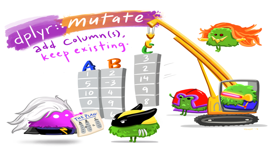
Artwork by @allison_horst
Within one mutate statement
Instant availability
Use new variables in the same function call right away!
# A tibble: 188 × 160
   mood_pre mood_post mood_change mood_change_norm start_date end_date  finished
      <dbl>     <dbl>       <dbl>            <dbl> <chr>      <chr>        <dbl>
 1       66         0         -66             9.12 11/3/2014  11/3/2014        1
 2       77        22         -55             7.60 11/4/2014  11/4/2014        1
 3       47       100          53             7.32 11/5/2014  11/5/2014        1
 4       25        72          47             6.49 11/4/2014  11/4/2014        1
 5       22        69          47             6.49 11/5/2014  11/5/2014        1
 6       37        83          46             6.36 11/6/2014  11/6/2014        1
 7       20        62          42             5.80 11/6/2014  11/6/2014        1
 8       60       100          40             5.53 11/4/2014  11/4/2014        1
 9       22        60          38             5.25 11/3/2014  11/3/2014        1
10       30        68          38             5.25 11/3/2014  11/3/2014        1
# ℹ 178 more rows
# ℹ 153 more variables: condition <chr>, subject <dbl>, gender <chr>,
#   age <dbl>, STAI_pre_1_1 <dbl>, STAI_pre_1_2 <dbl>, STAI_pre_1_3 <dbl>,
#   STAI_pre_1_4 <dbl>, STAI_pre_1_5 <dbl>, STAI_pre_1_6 <dbl>,
#   STAI_pre_1_7 <dbl>, STAI_pre_2_1 <dbl>, STAI_pre_2_2 <dbl>,
#   STAI_pre_2_3 <dbl>, STAI_pre_2_4 <dbl>, STAI_pre_2_5 <dbl>,
#   STAI_pre_2_6 <dbl>, STAI_pre_2_7 <dbl>, STAI_pre_3_1 <dbl>, …
na.rm = TRUE for computing mean after removing missing data
Replacing columns
Update existing
Using existing columns updates their content.
- Code lines 2 and 3
Warning
If not using names actions are used as names (avoid) - Code line 4
mutate() existing columns, centering mood columns
# A tibble: 188 × 3
   mood_pre mood_post `mood_pre - mean(mood_post, na.rm = TRUE)`
      <dbl>     <dbl>                                      <dbl>
 1   21.6       NA                                        21.6
 2   -0.358    -19.8                                      -0.358
 3  -37.4       -1.76                                    -37.4
 4   -6.36       6.24                                     -6.36
 5  -11.4       NA                                       -11.4
 6   13.6       11.2                                      13.6
 7   NA         NA                                        NA
 8   40.6       NA                                        40.6
 9    7.64      12.2                                       7.64
10  -29.4        6.24                                    -29.4
# ℹ 178 more rows
Replacing/recoding values (replace v1.2.0)
- Recoding creates a new column using values from an existing column (can be different data types)
- Replacing updates an existing column with new values. Same data type
| Recoding | Replacing | |
|---|---|---|
| Match with conditions | case_when() |
replace_when() |
| Match with values | recode_values() |
replace_values() |
Details in the vignette about recoding/replacing
Switch statement case_when() or replace some observations
Categorize mood_pre. Tests come sequentially.
# A tibble: 188 × 2
   mood_pre mood_pre_cat
      <dbl> <chr>
 1       81 exceptional
 2       59 great
 3       22 poor
 4       53 great
 5       48 mid
 6       73 great
 7       NA missing data
 8      100 exceptional
 9       67 great
10       30 mid
# ℹ 178 more rows
.unmatched = "error" would be better if you are sure to cover all cases (v1.2.0)
Cap bottom and top values. Using characters raises an error.
Your turn!
Create a new STAI_pre_category column.
Use case_when() to categorize values in STAI_pre as low, normal or high.
- For values < 25 in
STAI_preassign low - For values > 64 assign high
- For all other values assign normal.
Hint
To easily see the new column, use relocate() to move it to the first position of the tibble
Solution
# A tibble: 188 × 159
   STAI_pre_category STAI_pre start_date end_date  finished condition subject
   <chr>                <dbl> <chr>      <chr>        <dbl> <chr>       <dbl>
 1 normal                  32 11/3/2014  11/3/2014        1 control         2
 2 normal                  49 11/3/2014  11/3/2014        1 stress          1
 3 high                    65 11/3/2014  11/3/2014        1 stress          3
 4 normal                  42 11/3/2014  11/3/2014        1 stress          4
 5 normal                  33 11/3/2014  11/3/2014        1 control         7
 6 normal                  34 11/3/2014  11/3/2014        1 stress          6
 7 normal                  32 11/3/2014  11/3/2014        1 control         5
 8 low                     21 11/3/2014  11/3/2014        1 control         9
 9 normal                  31 11/3/2014  11/3/2014        1 stress         16
10 normal                  60 11/3/2014  11/3/2014        1 stress         13
# ℹ 178 more rows
# ℹ 152 more variables: gender <chr>, age <dbl>, mood_pre <dbl>,
#   mood_post <dbl>, STAI_pre_1_1 <dbl>, STAI_pre_1_2 <dbl>,
#   STAI_pre_1_3 <dbl>, STAI_pre_1_4 <dbl>, STAI_pre_1_5 <dbl>,
#   STAI_pre_1_6 <dbl>, STAI_pre_1_7 <dbl>, STAI_pre_2_1 <dbl>,
#   STAI_pre_2_2 <dbl>, STAI_pre_2_3 <dbl>, STAI_pre_2_4 <dbl>,
#   STAI_pre_2_5 <dbl>, STAI_pre_2_6 <dbl>, STAI_pre_2_7 <dbl>, …
Before we stop
You learned to:
- Selection and manipulation of
- observations,
- variables and
- values
Next step: Grouping and Summarizing
Acknowledgments 🙏 👏
- Lise Vaudor nice blog
- Allison Horst for the great ArtWork
- Jenny Bryan
- poorman by Nathan Eastwood, a re-implementation of
dplyrin base only
Contributions
- Milena Zizovic
- Roland Krause
- Veronica Codoni
Thank you for your attention!
![]()