Datasaurus

This guided practical will demonstrate that the tidyverse allows to compute summary statistics and visualize datasets efficiently. This dataset is already stored in a tidy tibble, cleaning steps will come in future practicals.

Those squared questions are optional

datasauRus package

Check if you have the package datasauRus installed

library(datasauRus)

Note

It should return nothing. If there is no package called ‘datasauRus’ appears, it means that the package needs to be installed. Use this in the console (will prevent the knit process otherwise):

install.packages("datasauRus")

Explore the dataset

Since we are dealing with a tibble, we can type

datasaurus_dozen

Only the first 10 rows are displayed.

# A tibble: 1,846 × 3
   dataset     x     y
   <chr>   <dbl> <dbl>
 1 dino     55.4  97.2
 2 dino     51.5  96.0
 3 dino     46.2  94.5
 4 dino     42.8  91.4
 5 dino     40.8  88.3
 6 dino     38.7  84.9
 7 dino     35.6  79.9
 8 dino     33.1  77.6
 9 dino     29.0  74.5
10 dino     26.2  71.4
# ℹ 1,836 more rows

What are the dimensions of this dataset? Rows and columns?

• base version, using either dim(), ncol() and nrow()

Solution

# dim() returns the dimensions of the data frame, i.e number of rows and columns
dim(datasaurus_dozen)

[1] 1846    3

# ncol() only number of columns
ncol(datasaurus_dozen)

[1] 3

# nrow() only number of rows
nrow(datasaurus_dozen)

[1] 1846

• tidyverse version

Solution

nothing to be done, a tibble display its dimensions, starting by a comment (‘#’ character)

Assign the datasaurus_dozen to the ds_dozen name. This aims at populating the Global Environment

Solution

ds_dozen <- datasaurus_dozen

Using Rstudio, those dimensions are now also reported within the interface, where?

Solution

in the Environment panel -> Global Environment

How many datasets are present?

• base version

Tip

You want to count the number of unique elements in the column dataset. The character $ applied to a data.frame subset the column and convert the 2D structure to 1D, i. e a vector. The function length() returns the length of a vector, such as the unique elements

Solution

length(unique(ds_dozen$dataset))

[1] 13

• tidyverse version

# n_distinct counts the unique elements in a given vector.
# we use summarise to return only the desired column named n here.
# we use English verbs and no subsetting characters, nor we change dimensions (keep a tibble)
summarise(ds_dozen, n = n_distinct(dataset))

# A tibble: 1 × 1
      n
  <int>
1    13

• even better, compute and display the number of lines per dataset

Tip

the function count in dplyr does the group_by() by the specified column + summarise(n = n()) which returns the number of observation per defined group.

Solution

count(ds_dozen, dataset)

# A tibble: 13 × 2
   dataset        n
   <chr>      <int>
 1 away         142
 2 bullseye     142
 3 circle       142
 4 dino         142
 5 dots         142
 6 h_lines      142
 7 high_lines   142
 8 slant_down   142
 9 slant_up     142
10 star         142
11 v_lines      142
12 wide_lines   142
13 x_shape      142

Check summary statistics per dataset

Compute the mean of the x & y column. For this, you need to group_by() the appropriate column and then summarise()

Tip

in summarise() you can define as many new columns as you wish. No need to call it for every single variable.

Solution

ds_dozen |>
  summarise(mean_x = mean(x),
            mean_y = mean(y), .by = dataset)

# A tibble: 13 × 3
   dataset    mean_x mean_y
   <chr>       <dbl>  <dbl>
 1 dino         54.3   47.8
 2 away         54.3   47.8
 3 h_lines      54.3   47.8
 4 v_lines      54.3   47.8
 5 x_shape      54.3   47.8
 6 star         54.3   47.8
 7 high_lines   54.3   47.8
 8 dots         54.3   47.8
 9 circle       54.3   47.8
10 bullseye     54.3   47.8
11 slant_up     54.3   47.8
12 slant_down   54.3   47.8
13 wide_lines   54.3   47.8

Compute both mean and standard deviation (sd) in one go using across()

Solution

ds_dozen|>
  # across works with first on which columns and second on what to perform on selection
  # 2 possibilities to select columns
  # summarise(across(where(is.double), list(mean = mean, sd = sd)))
  # by default in 1.0.5, grouped variables are excluded from across
  # summarise(across(everything(), list(mean = mean, sd = sd)))
  summarise(across(c(x, y), list(mean = mean, sd = sd)),
            .by = dataset)

# A tibble: 13 × 5
   dataset    x_mean  x_sd y_mean  y_sd
   <chr>       <dbl> <dbl>  <dbl> <dbl>
 1 dino         54.3  16.8   47.8  26.9
 2 away         54.3  16.8   47.8  26.9
 3 h_lines      54.3  16.8   47.8  26.9
 4 v_lines      54.3  16.8   47.8  26.9
 5 x_shape      54.3  16.8   47.8  26.9
 6 star         54.3  16.8   47.8  26.9
 7 high_lines   54.3  16.8   47.8  26.9
 8 dots         54.3  16.8   47.8  26.9
 9 circle       54.3  16.8   47.8  26.9
10 bullseye     54.3  16.8   47.8  26.9
11 slant_up     54.3  16.8   47.8  26.9
12 slant_down   54.3  16.8   47.8  26.9
13 wide_lines   54.3  16.8   47.8  26.9

What can you conclude?

Solution

all mean and sd are the same for the 13 datasets

Plot the datasauRus

Plot the ds_dozen with ggplot such the aesthetics are aes(x = x, y = y)

with the geometry geom_point()

Tip

the ggplot() and geom_point() functions must be linked with a + sign

Solution

ggplot(ds_dozen, aes(x = x, y = y)) +
  geom_point()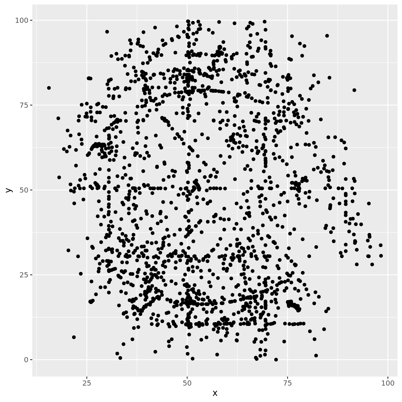

Reuse the above command, and now colored by the dataset column

Solution

ggplot(ds_dozen, 
       aes(x = x, 
           y = y, 
           colour = dataset)) +
  geom_point()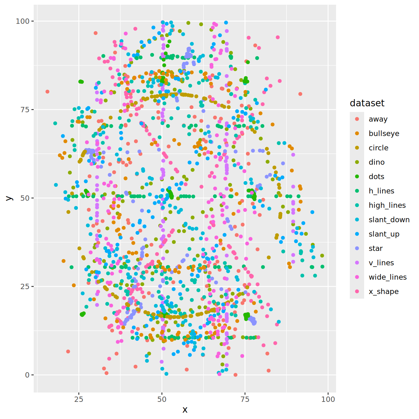

Too many datasets are displayed.

How can we plot only one at a time?

Tip

You can filter for one dataset upstream of plotting

Solution

ds_dozen|>
  filter(dataset == "away")|>
  ggplot(aes(x = x, y = y)) +
  geom_point()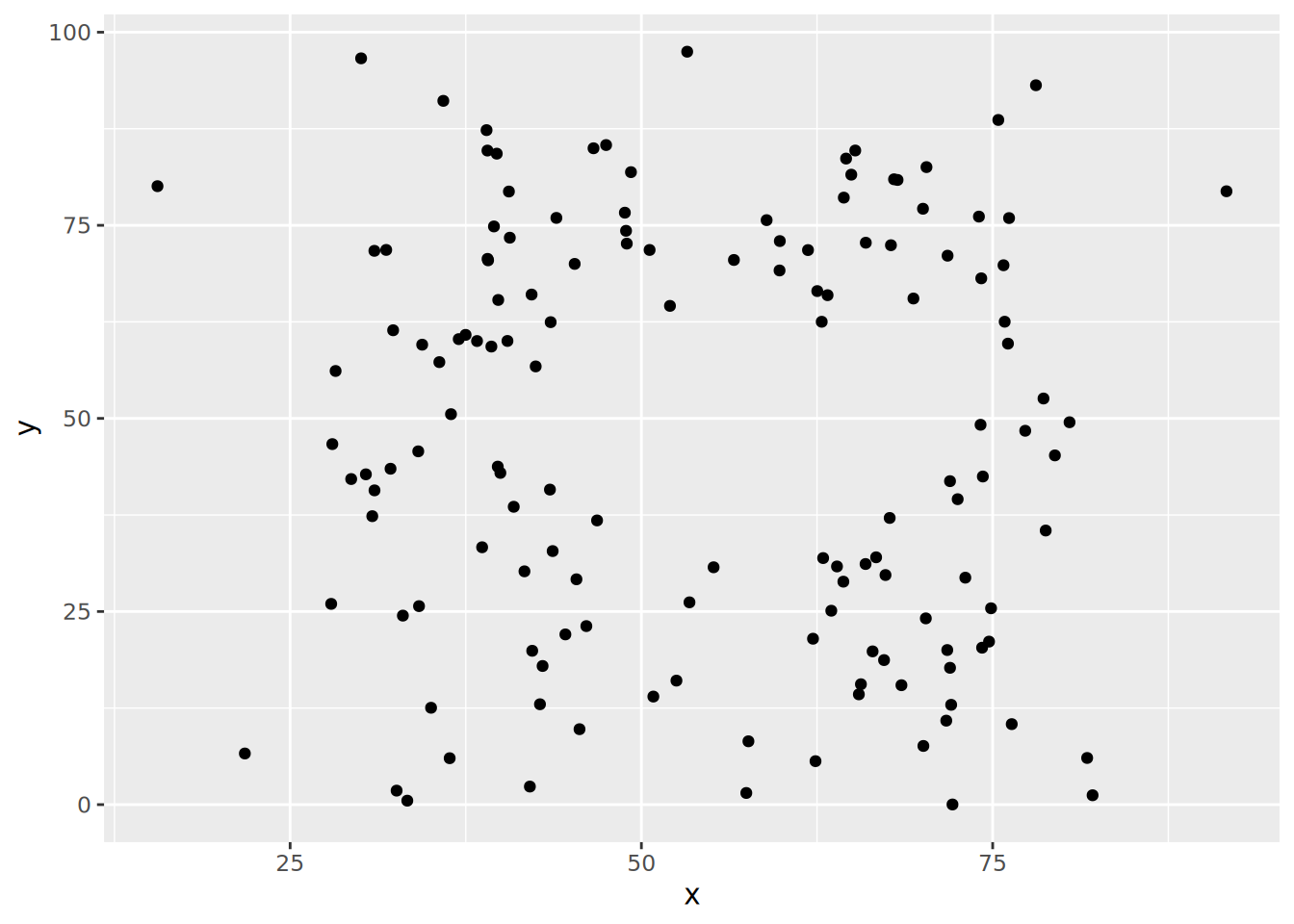

Adjust the filtering step to plot two datasets

Tip

R provides the inline instruction %in% to test if there a match in the left operand with the right one (a vector most probably)

Solution

ds_dozen|>
  filter(dataset %in% c("away", "dino"))|>
  # alternative without %in% and using OR (|)
  #filter(dataset == "away" | dataset == "dino")|>
  ggplot(aes(x = x, y = y, colour = dataset)) +
  geom_point()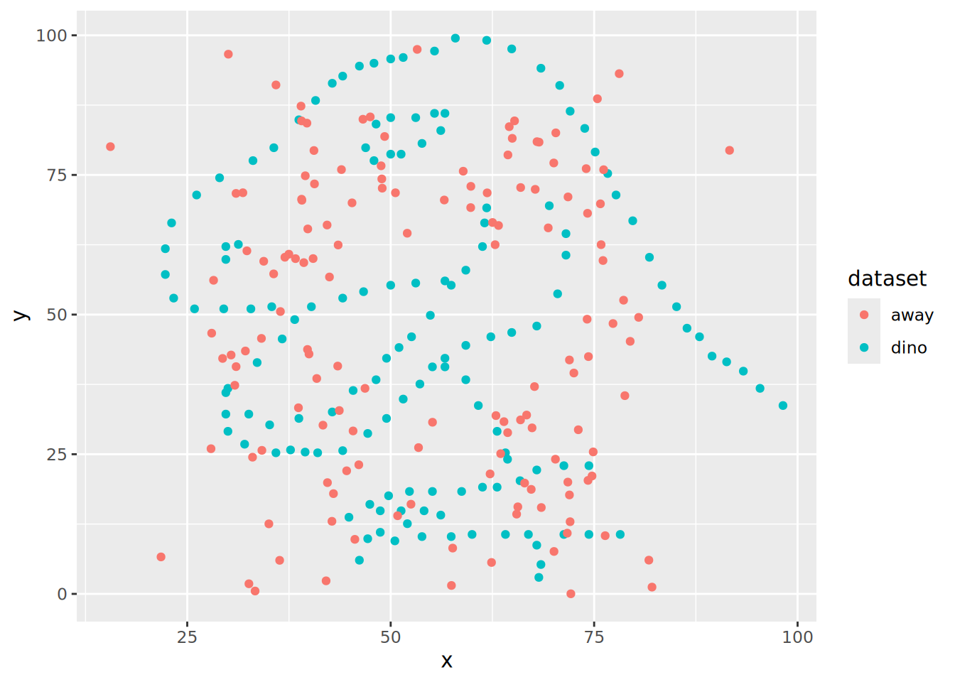

Expand now by getting one dataset per facet

Solution

ds_dozen|>
  filter(dataset %in% c("away", "dino"))|>
  ggplot(aes(x = x, y = y, colour = dataset)) +
  geom_point() +
  facet_wrap(vars(dataset))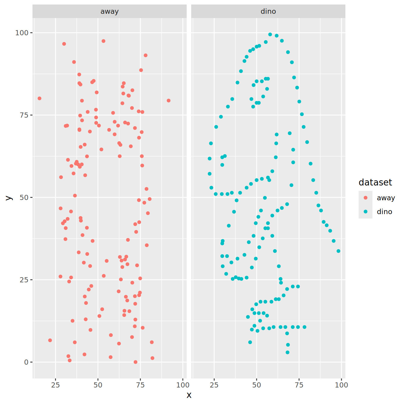

Remove the filtering step to facet all datasets

Solution

ds_dozen|>
  ggplot(aes(x = x, y = y, colour = dataset)) +
  geom_point() +
  facet_wrap(vars(dataset), ncol = 3)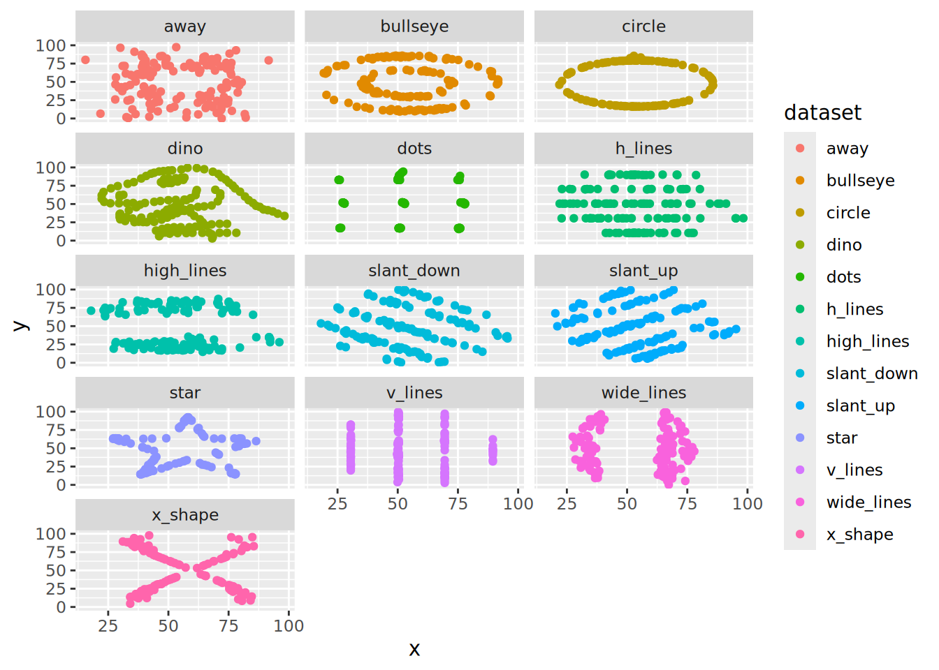

Tweak the theme and use the theme_void() and remove the legend

Solution

ggplot(ds_dozen, aes(x = x, y = y, colour = dataset)) +
  geom_point() +
  theme_void() +
  theme(legend.position = "none") +
  facet_wrap(vars(dataset), ncol = 3)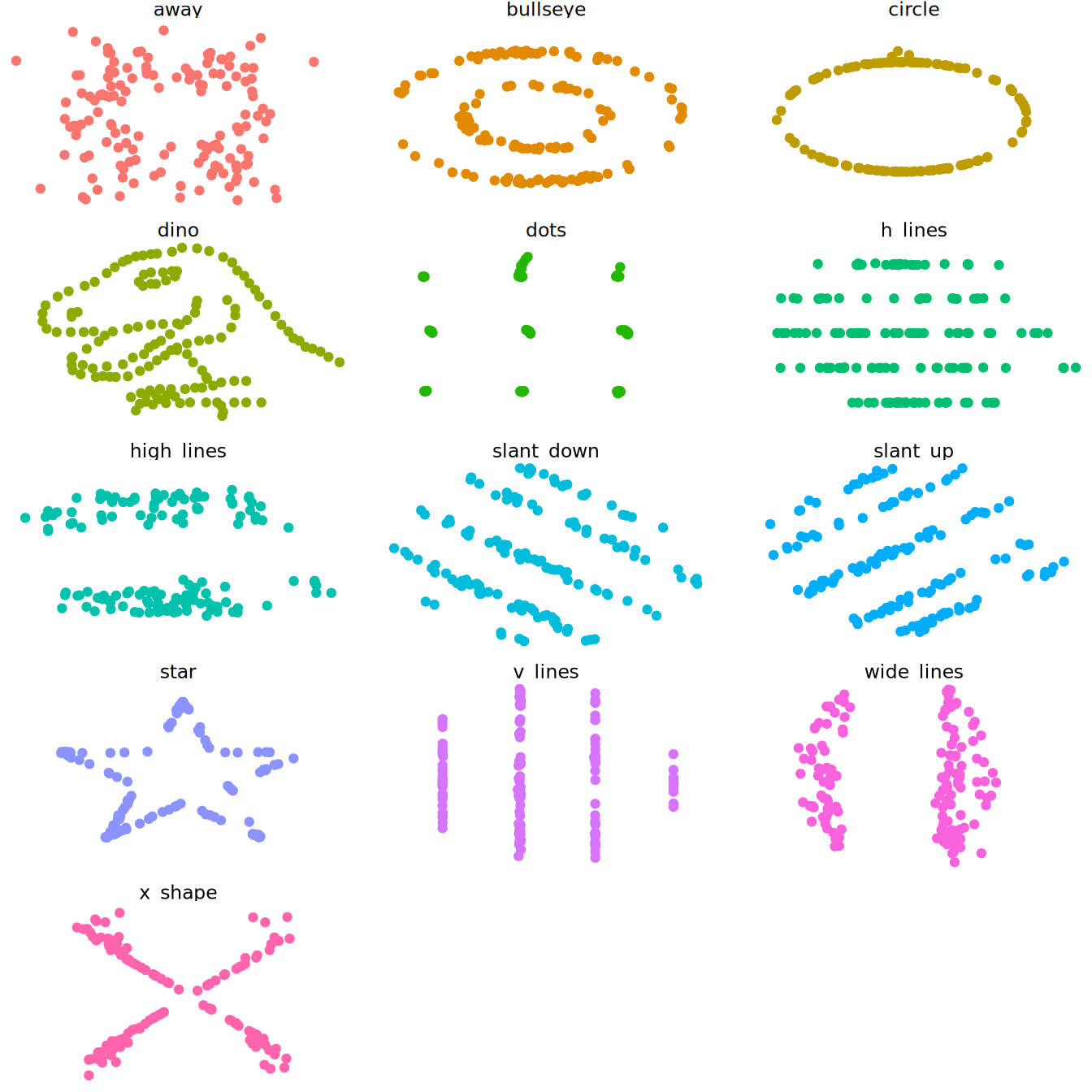

Are the datasets actually that similar?

Solution

No ;) We were fooled by the summary stats

Animation

Plots can be animated, see for example what can be done with gganimate. Instead of panels, states are made across datasets and transitions smoothed with an afterglow effect.

Solution

Conclusion

Never trust summary statistics alone; always visualize your data | Alberto Cairo

Authors

• Alberto Cairo, (creator)
• Justin Matejka
• George Fitzmaurice
• Lucy McGowan

from this post