Check on published results concerning the relationship between a gene and a microRNA in colon cancer
Those kind of questions are optional
Microarray analysis
We will be working with GEO datasets, places where submitting microarray experiments is required by most journals. You will experience that despite being around for many years, manipulating those data can be a hassle.
Here, we will investigate the relationship between the expression of ENTPD5 and mir-182 as it was described by Pizzini et al.. Even if the data are already normalised and should be ready to use, you will see that reproducing the claimed results can be tedious.
Load the study using the file gse35834.rds using read_rds(). Save as gse35834
TipTip
RDS are R binary format. Bioconductor objects are not flat files but complex structures (cf scheme below). Thus, we need to use this binary format to load them. The function readr::read_rds() recognises this format.
Of note, we could use GEOquery to fetch directly from NCBI but it is not always available.
What kind of object is gse35834?
TipTip
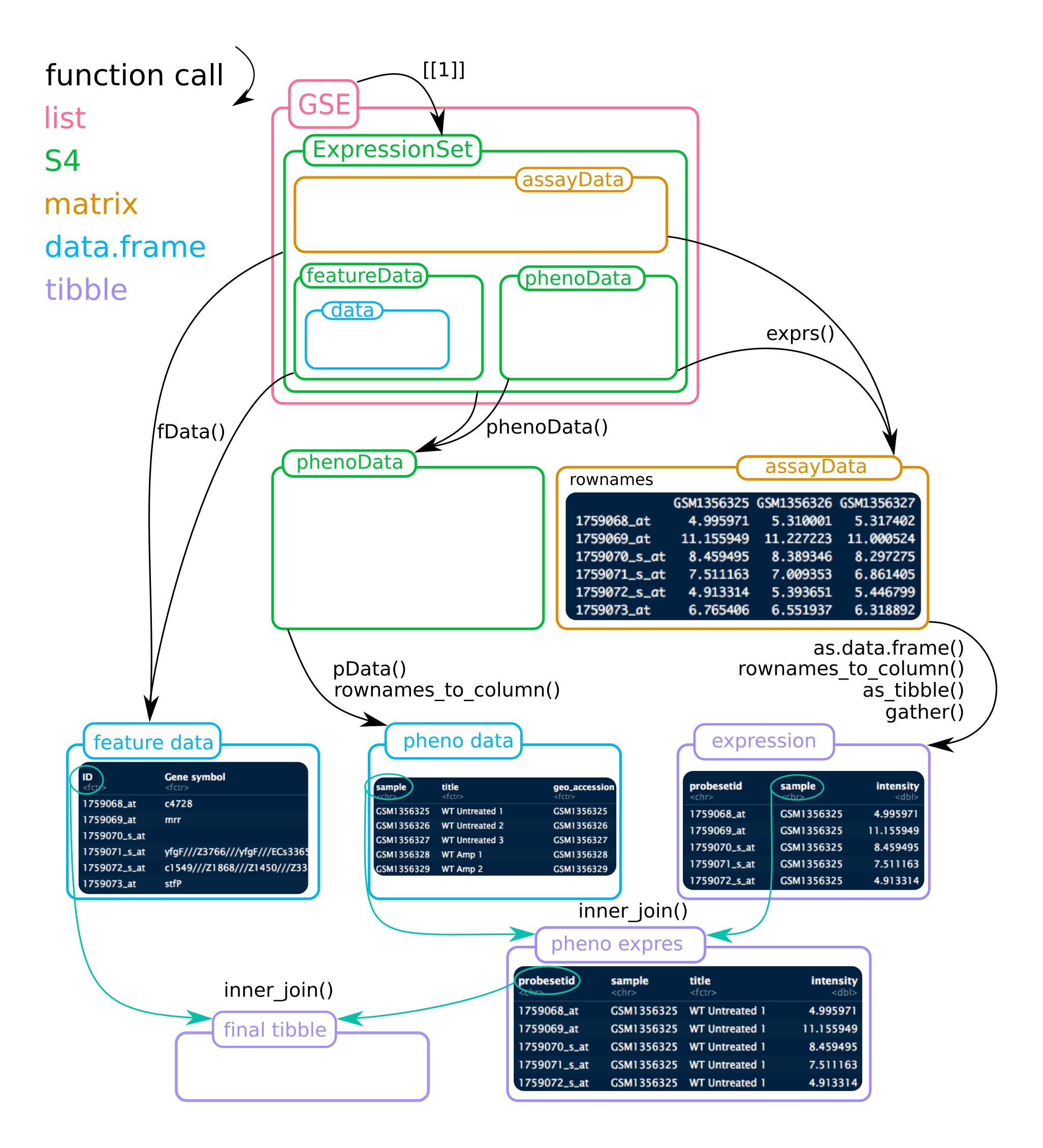
To help figuring out the ExpressionSet object, see the figure below. Mind that for this project, the list GSE contains 2 ExpressionSets!
Figure 1
Two expression platforms were used in this study, which ones according to the main page GSE35834?
Tidying ExpressionSet objects
Before the infusion of the tidyverse in Bioconductor, we needed to perform all the operations described in Figure 1 in order to obtain a tibble where metadata (both about patients and genes) and expressions values are together. Hopefully, this is simplified now thanks to tidySummarizedExperiment and Stefano Mangiola work.
How can you extract the mRNA or mir data to each element of gse35834?
TipTip
The object is a list, each sub-object is the ExpressionSet we need to access. For example, gse35834[[1]] will sub-select and extract (so the double square brackets) for the mRNA platform
Apply the function makeSummarizedExperimentFromExpressionSet from tidySummarizedExperiment to the RNA part of gse35834. Assign the name tidy_rna
NoteExtension of tibble to Bioconductor objects
You can see now that by calling the object tidy_rna, that the embedded tibble is ~ 1.8M rows but the SummarizedExperiment contains 22,846 features (= genes) and 80 samples. The samples (.sample) were already pivoted to the long format
# A SummarizedExperiment-tibble abstraction: 1,798,880 × 55# Features=22486 | Samples=80 | Assays=exprs .feature .sample exprs title geo_accession status submission_date last_update_date type channel_count source_name_ch1 <chr> <chr> <dbl> <fct> <chr> <fct> <fct> <fct> <fct> <fct> <fct> 1 10000_at GSM875933 5.86 exon… GSM875933 Publi… Feb 15 2012 Jan 16 2014 RNA 1 colon cancer, … 2 10001_at GSM875933 6.60 exon… GSM875933 Publi… Feb 15 2012 Jan 16 2014 RNA 1 colon cancer, … 3 10002_at GSM875933 5.43 exon… GSM875933 Publi… Feb 15 2012 Jan 16 2014 [...]
Apply the function makeSummarizedExperimentFromExpressionSet from tidySummarizedExperiment to the microRNA part of gse35834. Assign the name tidy_mir
Explore and merge both expression meta-data
mRNA and mir meta-data
Extract the mRNA meta-data as a tibble to which you assign the name rna_meta.
TipTip
To be consistent, follow those two guidelines:
Convert the SummarizedExperiment to a tibble with as_tibble()
Retain only the columns .feature, .sample, exprs, source_name_ch1 and
characteristics_ch1 rename to gender
characteristics_ch1.1 rename to patient
Extract the mir expression meta-data similarly. Save as mir_rna
Filter RNA expression data for the ENTPD5 gene
For the microRNA, the .feature contains the mir names, however for the mRNA, we only have the probeset ids. We need one more step to extract only the expression of the desired gene.
featureData can be accessed, and for example the first line for mRNA:
Join the expression data rna_meta to the platform annotations (fData(gse35834[[1]])). Assign the name rna_expression_feature
Filter rna_expression_feature for the gene of interest (ENTPD5). Assign the name rna_expression_entpd5.
TipTip
At this point you should get a tibble of 80 values and 9 columns
Join with the mir expression data
In both tibbles, are the samples identifiers (GSM[...]) identical?
To join tables, we need one or more common key(s). We would like to somehow join both information.
Knowing that both data frames have different sample columns,
Merge both meta-data to get the correspondences between RNAGSM* and mirGSM*. Save the result as rna_entpd5_mir.
ImportantWarning
To be clear, you MUST use specify by which columns you join both tables and NOT include the column .sample. Since it exists in both tables and have nothing in common.
TipTip
When tables are joined by specific columns, remaining columns that have identical names get default suffixes ‘.x’ and ‘.y’ appended. However, you can make more friendly suffixes that match your actual data using the suffix = c("_rna", "_mir")
Filter for the miR-182 from rna_entpd5_mir. Assign the name rna_entpd5_mir_182
TipTip
Filter for the mir of interest: hsa-miR-182_st (hsa = Homo sapiens)
We discard the complementary hsa-miR-182-start_st
How many rows do you obtain? How many are expected?
Find the discrepancy, write down the missing GSM sample but proceed anyway.
TipTip
anti_join() returns the NON match keys.
Examine gene expression according to some meta data
Plot the gene expression distribution by Gender. Is there any obvious difference?
TipTip
boxplots are one option, but we get so much more information using: