Voyager Golden Record

Author

Aurélien Ginolhac

Published

June 30, 2026

Objective

Decode all images from the Golden Record attached to the Voyager spacecrafts

Those squared questions are optional

Context

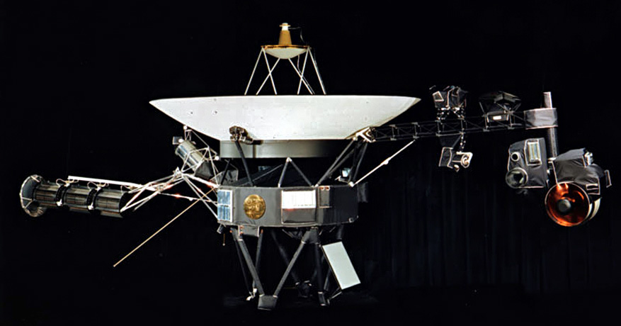
In 1977, two spacecrafts named Voyager 1 and 2 were launched from Earth to explore mostly Jupiter and Saturn for Voyager 1 and Uranus and Neptune for Voyager 2. Today, they are more than 24 billions kilometers from us, reaching the interstellar space in 2012. Recently (in June 2024), Voyager 1 and the scientists were able to communicate again and get data from 4 instruments (out of 10).

The Golden Record

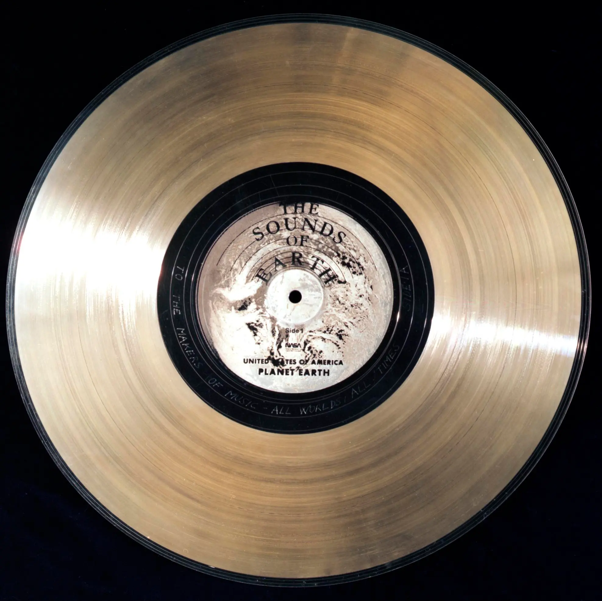
The contents of the golden record were selected for NASA by a committee led by Carl Sagan of Cornell University.

The record is constructed of gold-plated copper and is 30 cm in diameter. The record’s cover is aluminum and electroplated upon it is an ultra-pure sample of the isotope uranium-238. Uranium-238 has a half-life of 4.468 billion years (to determined construction date).

Greetings in 55 languages
Music, 19 tracks, Bach, Chuck Berry, traditional songs
Pictures: 115 images

Decoding instructions

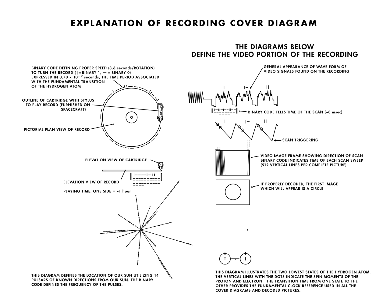
Engraved on the gold cover, and stylus is included on the spacecraft. Expected speed rotation is 3.6 seconds, related to the di-hydrogen atom spin.

Encoded images

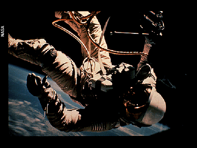
The NASA dedicated page provides only 48 images / 115. Rest cannot be seen:

Due to copyright restrictions, only a subset of the images on the Golden Record are displayed above.

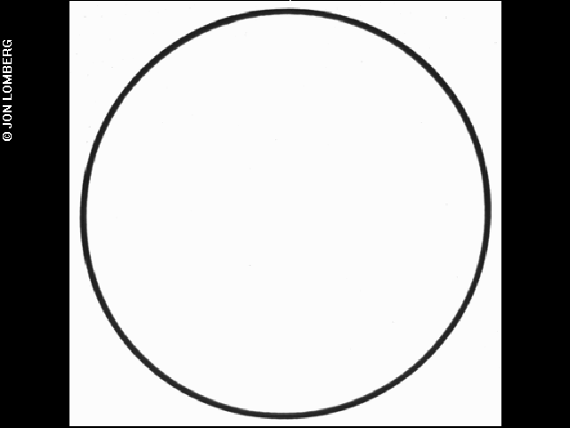
The calibration circle that the alien should first see if they decode it correctly.

Music source

Ozma Records proposes the Vinyl Set with a link the music tracks on SoundCloud.

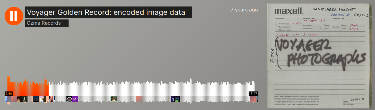
Both the MP3 (17.7 MB) and WAV (1.4 GB) format are available on the Internet. Watch out that the sample rate is different, 44.1kHz and 384kHz respectively.

Decoding images

The stereo signal from the WAV file needs to be turns into some tables, and those steps were spared to you. The two audio channels, left and right were cleaned from a noise tone, and both channels saved as an indexed tibble of two columns (left and right).

The file is channels_no_tone.fst (2.7GB), so in a format that allows the great feature of random access of the {fst} package.

Random access means you can instantly access some slices of a large file as long as you know where to start and stop.

What was done for you upfront is to:

Read in signal from the Audio file, rate is 384000 (number of values for 1 second). Total length is less than 8 minutes and encode 154 images.
Normalize both left and right channels to their maximum absolute values
Remove[^It was done by finding the 5% most down peaks in the first 30 seconds] a big noise tone at the beginning (you can listen to it on SoundCloud how unpleasant it is), as seen below (example from the left channel)
Find images indexes on both channels

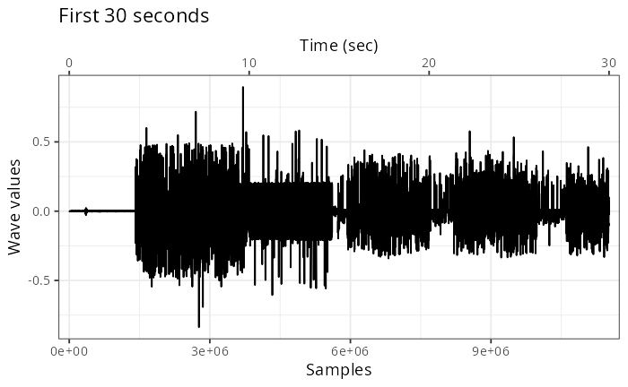
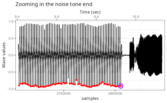
The left image shows the first 30 seconds, the right one zoom on 9-11 seconds.

Roughly from 4 seconds to 10 seconds consist in highly oscillating noise. You can also observe the detection of peaks (in red, and the last one circled in purple) using the R package {pracma}.

The same procedure will be need to detect each image, and inside, each image line. Piling up signal for each lines in a matrix will allow to create the image after some conversion in 0-255 grey scale.

Install the `fst` package

Once we have the start and end of each image, one can slice from the Fast Serialize data frame full file really fast (it is also multi-threaded).

Download locally necessary files

The light fst file, normalized signals of the first 8 images (2 channels) (288MB)
The full fst file, normalized data of +70 images (2 channels) (2.7GB)
The tsv file, indexes of where each image starts on each channel (1.5KB)

The goal of having both a light and full signal is to work first with light one, obtain the first images, then use the full to see all images.

For a first time, download locally the light fst file. This file path string will be referred to with the name voyager_fst. You can read it with fst::read_fst(voyager_fst).

You should obtain a data.frame of 19,978,488 rows × 2 columns: left and right.

The image indexes, i.e where exactly each image starts from the signal are in a small TSV, 77 rows for 2 columns, left and right

Confirming the indexing on the first 3 images

To see globally how the images are encoded (remember this was done in 1976!) and if the indexes of image start are correct, let’s assess it on the first 3 images of the left channel. to achieve this, we focus on the seconds 10 to 30 of the recording. The first 10 seconds were removed as they are just noise but we need to keep the index in sync to offset correctly.

What we mean by index

Each row of the signals, on both channels is a sample, every rate (384,000) rows is equal to 1 second. And since we have a fst file, we can slice instantly the rows we want. If we have the start index of image 2 and 3, one can extract the signal using

fst::read_fst(voyager)

Here is the index of the noisy tone ending, and sampling rate:

noisy_tone_end <- 3810661
rate <- 384000

Plot the Signal values in function of time for 10-30 seconds, highlighting with vertical bars the start of the 3 images

Create a tibble with one column y, the left signal, sliced from row 1 to 7296000 (19 sec * rate):

fst::read_fst(voyager_fst, 
              columns = "left", 
              from = 1, to = 7296000) |> pull()

Add a second column x with row_number() + noisy_tone_end, creating integers from 3,810,662 to 11,106,661 to include the shift of the noise trimming
(Optional) Sample randomly only 1e6 lines to save some plotting time using slice_sample(n = 1e6)
Plot y ~ x with lines
Add vertical lines with geom_vline() where the data is a tibble of x = img_indexes$left[1:3]) + noisy_tone_end to get indexes of first 3 images
(Optional) Add a secondary x-axis to have the time in seconds:

  scale_x_continuous(sec.axis = sec_axis(\(x) x / rate, name = "Time (sec)"))

How to interpret the signal and the vertical indexes of image starts?

Composition of one image

In between two image indexes, we have signal but what is it exactly? It consists of line in which we the values of pixels. Meaning that if we fill a matrix of all image lines in columns for example, and for each line, the rows are values, we end up with one matrix per image, that R can display natively.

The lines are actually smaller indexes within one image, with a higher peak indicating we switch to a new line.

In order to find peaks within an image, we must first have a function that extract the signal values for it. This function should take two arguments, the positive integer of the image (from 1 to 77) and a string, either "left" or "right". Then we can extract the signal of the 154 images from both channels.

Write a function named `extract_img_signal()` that takes two arguments: `index` and `channel` and return the data vector of the desired image

channel should be either "left" or "right"
index should be an integer from 1 to 77
Slice the voyager_fst file with the appropriate index and channel from the tibble img_indexes
Pull out the vector of values.

Note

The resulting vector for one image should around 2 millions values of float numbers

For example, the length of vectors for the 8 first images (light fst file don’t have more) on the left channels are:

Tip integer

1 is actual a double, so a float number. To specify in R you meant an integer, add L after the digit

1L

[1] 1

is.integer(3L)

[1] TRUE

From the `{pracma}` R package, use the function `findPeaks()` to find lines for one image

Let’s define img_signal the output of the previous function like: img_signal <- extract_img_signal(channel = "left", index = 1L)
The following code

library(pracma) # needed only once in your document
findpeaks(img_signal,
          minpeakheight = 0.05,
          minpeakdistance = rate / 100) |> 
  as.data.frame() |> 
  as_tibble() |> 
  arrange(V2)

should give:

# A tibble: 358 × 4
      V1    V2    V3    V4
   <dbl> <dbl> <dbl> <dbl>
 1 0.656  3096  3091  3100
 2 0.365  8527  8507  8537
 3 0.897 12793 12772 12797
 4 0.366 17981 17954 17992
 5 0.910 22282 22262 22286
 6 0.366 28013 27994 28022
 7 0.630 31969 31957 31972
 8 0.464 41464 41450 41468
 9 0.410 47861 47852 47865
10 0.534 54251 54244 54254
# ℹ 348 more rows

Where the column V2 is the index of each line start.

Encapsulate the previous code in a function called `find_row_indexes` that takes an image signal vector and returns a 4 column tibble from findPeak

Check this row indexing on the quarter of the first image

Start from the same plot as confirming the first 3 indexes of images, but using img_signal so within now a single image. The first one of the left channel. Actually, this should the calibration circle that should allow aliens to know they are one the right track decoding the Golden Record. Now, you are the alien and on this plot, you should be able to see the circle already at this stage be stretching horizontally the plot.

Keep only the row numbers < 1.5e6
For the geom_vline() data are the row_index tibble, filtered for < 1.5e6 and mapping: xintercept = V2

Create the image and visualize it

The toolbox we have in hands are:

A fst file in which we can slice efficiently any image values, with relevant indexes of our choice with extract_img_signal()
A function find_row_indexes() that find where each image line start

Now we need to fill in a matrix for each image line with the image values.

The constants used were discovered empirically by Brandon Moore

SCANWIDTH <- 3000
BORDERS <- 10

Write a function `fill_img_matrix` that takes an image signal and returns the filled matrix one row per line

The first step is call the function find_row_indexes and assign the name row_index
Initialize a matrix at the correct dimensions with the following:

    img_data <- matrix(nrow = length(row_index$V2), ncol = (SCANWIDTH))

For each row, starting from 1, iterate through the row_index$V2
- Extract the line from img_signal
- Fill the matrix for the relevant row with the extracted values
- Increment the row variable for the next for loop iteration
When matrix is fill up, return it, and let’s see its name is img_data
Display with: image(img_data, col = gray.colors(255))

You should see the calibration circle!

Tip

There are some improvements that can be run:

Rescale values to be between 0 and 255
Clip off borders
Clip off extreme values based on quantiles (2 and 98%)
Remove lines with no meaningful data

But without it’s enough to see the images. Ask me if you want to implement those improvements.

At least rescaling values is the one to do first to fit the 255 grey scale.

To recap, you can now display any images with the following snippet, for example to see the third image on the right channel:

extract_img_signal(channel = "right", index = 3L) |>
  fill_img_matrix() |> 
  image(col = gray.colors(255))

Plot the image with ggplot2. Implies to convert matrix to tibble and pivot to the longer format

The geom to use is geom_raster()
Force grey scale with scale_fill_gradient(low = "white", high = "grey30")
To get image in the right sense: scale_y_continuous(transform = "reverse")
Clean up annotation with theme_void()

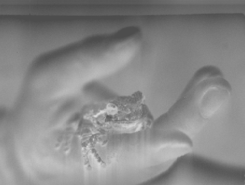
See one output: frog in a hand.

Color images

Some images are in colors and were encoded then 3 times, the red, green and blue channels.

For example, on the left channel, images 8, 9 and 10 are the Sun spectra. Images 45, 46 and 47 are a son on his Dad’ shoulders.

Once the 3 rescaled matrices are obtained, one can mingled them with rgb() and display them with rasterImage() but I got some unresolved shifts so far.

Acknowledgments 🙏 👏

Carl Sagan and JPL/Caltech Team
Ron Barry for his inspiring article.
Brandon Moore for easy to follow Python code.
Baptiste for creating rgb color images.

Those squared questions are optional

Context

The Golden Record

Decoding instructions

Encoded images

Music source

Decoding images

Install the fst package

Download locally necessary files

Confirming the indexing on the first 3 images

Plot the Signal values in function of time for 10-30 seconds, highlighting with vertical bars the start of the 3 images

Composition of one image

Write a function named extract_img_signal() that takes two arguments: index and channel and return the data vector of the desired image

From the {pracma} R package, use the function findPeaks() to find lines for one image

Encapsulate the previous code in a function called find_row_indexes that takes an image signal vector and returns a 4 column tibble from findPeak

Check this row indexing on the quarter of the first image

Create the image and visualize it

Write a function fill_img_matrix that takes an image signal and returns the filled matrix one row per line

Plot the image with ggplot2. Implies to convert matrix to tibble and pivot to the longer format

Color images

Acknowledgments 🙏 👏

Install the `fst` package

Write a function named `extract_img_signal()` that takes two arguments: `index` and `channel` and return the data vector of the desired image

From the `{pracma}` R package, use the function `findPeaks()` to find lines for one image

Encapsulate the previous code in a function called `find_row_indexes` that takes an image signal vector and returns a 4 column tibble from findPeak

Write a function `fill_img_matrix` that takes an image signal and returns the filled matrix one row per line